Assessment of Solution Algorithms for LES of Turbulent Flows Using OpenFOAM

Abstract

We validate and test two algorithms for the time integration of the Boussinesq form of the Navier—Stokes equations within the Large Eddy Simulation (LES) methodology for turbulent flows. The algorithms are implemented in the OpenFOAM framework. From one side, we have implemented an energy-conserving incremental-pressure Runge–Kutta (RK4) projection method for the solution of the Navier–Stokes equations together with a dynamic Lagrangian mixed model for momentum and scalar subgrid-scale (SGS) fluxes; from the other side we revisit the PISO algorithm present in OpenFOAM (pisoFoam) in conjunction with the dynamic eddy-viscosity model for SGS momentum fluxes and a Reynolds Analogy for the scalar SGS fluxes, and used for the study of turbulent channel flows and buoyancy-driven flows. In both cases the validity of the anisotropic filter function, suited for non-homogeneous hexahedral meshes, has been studied and proven to be useful for industrial LES. Preliminary tests on energy-conservation properties of the algorithms studied (without the inclusion of the subgrid-scale models) show the superiority of RK4 over pisoFoam, which exhibits dissipative features. We carried out additional tests for wall-bounded channel flow and for Rayleigh–Bènard convection in the turbulent regime, by running LES using both algorithms. Results show the RK4 algorithm together with the dynamic Lagrangian mixed model gives better results in the cases analyzed for both first- and second-order statistics. On the other hand, the dissipative features of pisoFoam detected in the previous tests reflect in a less accurate evaluation of the statistics of the turbulent field, although the presence of the subgrid-scale model improves the quality of the results compared to a correspondent coarse direct numerical simulation. In case of Rayleigh–Bénard convection, the results of pisoFoam improve with increasing values of Rayleigh number, and this may be attributed to the Reynolds Analogy used for the subgrid-scale temperature fluxes. Finally, we point out that the present analysis holds for hexahedral meshes. More research is need for extension of the methods proposed to general unstructured grids.

1. Introduction

Since the seminal works of Chorin [1] and Temam [2], different variants of the fractional-step method have been proposed and used for the integration of the incompressible form of the unsteady Navier–Stokes Equations (NSE). Over the years, different algorithms have been developed using multistep time advancement techniques, conceived to be used with generalized grid topologies and different locations of the flow variables (co-located or staggered). Algorithms developed for the analysis of unsteady laminar flows have been successfully employed for the Direct Numerical Simulations (DNS) and for the Large Eddy Simulation (LES) of turbulent flows. The latter, by requiring some forms of parametrization for the smallest scales of turbulence, is computationally less demanding. In principle, even non-conservative or dissipative numerical algorithms may give reasonable results when used for DNS, provided that the time step of the simulation and the cell size are smaller than the Kolmogorov scales, so that the truncation error remains confined in the insignificant part of the power spectrum. This is not true for LES though, where a low-pass filter is applied to the NSE to separate the large energy-carrying scales of motion from the small and more isotropic ones; here the truncation error necessarily affects both the resolved and the modeled part of the spectrum, hence the importance of using energy-conserving and non-dissipative algorithms for LES of turbulent flow.

In a sequence of papers [3,4] numerical algorithms for the solution of the NSE in conservative form have been proposed, using Cartesian staggered grids. There, 2nd-order accurate central difference schemes were used for the discrete spatial operators, second-order time accurate schemes for the diffusive terms, and, at least second-order accurate schemes for time integration of the non-linear term (i.e., Adams–Bashforth or Runge–Kutta). The need to move toward complex grid topologies has pushed the development of algorithms using curvilinear coordinate transformations or unstructured grids. A very popular curvilinear-grid fractional-step algorithm is that of Zang et al. [5]: they used a semi-implicit time advancement scheme in conjunction with a second-order accurate explicit Adams–Bashforth scheme for the time integration of the non-linear term. Since the algorithm co-locates the flow variables on the cell centroids it requires a non-conservative formulation of the NSE [6] thus, high-order upwind flux schemes were used for the spatial discretization of the advective term of momentum and scalar transport. The algorithm was successfully employed for the study of LES of turbulent flows over curvilinear geometries. Later, the algorithm was modified using central differences for the calculation of non-linear momentum and scalar fluxes in several papers (see [7] for a general discussion). On the other side, energy-conserving, second-order fractional-step algorithms for finite-differences/volumes have been proposed and used for the LES of turbulent flows in unstructured grids [8].

Given the Courant-Friedrich-Lewis (CFL) restrictions imposed by the semi-explicit methods mentioned earlier, implicit multistep methods for the solution of the NSE were sought. In its incompressible version, the NSE present some difficulties in enforcing mass conservation and in writing the discrete non-linear operator of velocities when numerically integrated using implicit multistep methods. The most widely used algorithm for the implicit integration of the incompressible NSE is the PISO algorithm, proposed by Issa [9], which is first-order accurate in time. As it is a non-iterative predictor-corrector method, the  momentum equation (predictor) is solved once and, afterward, the non-solenoidal velocities obtained are ‘corrected’ (at least twice) in order to enforce conservation of mass, by solving the pressure equation and an explicit algebraic corrector equation. It is important to note that for the algorithm to be implicit, the advective term must be linearized. Details on such linearization will be revisited in later sections.

OpenFOAM [10,11,12] is a numerical library based on the idea of offering an unified mathematical framework for the description of systems of hyperbolic Partial Differential Equations (PDE) in a natural way, where the finite-volume (FV) approach is used for the ‘discretization’ of spatial derivative operators and where multistep time integration techniques are present. In particular, the PISO algorithm present in OpenFOAM, referred also as pisoFoam, has become a tool of widespread use in industry as well as in academia for the solution of the incompressible NSE. In academia, the code has been largely used for unsteady simulations using Detached Large Eddy, wall-resolving Large Eddy (A simulation where the near-wall turbulent structures are fully resolved and a no-slip boundary condition is applied at the wall), implicit Large Eddy (ILES) (a simulation where the SGS model is replaced by the truncation error of the numerical algorithm) models and more recently for DNS. There, it has proven to be the go-to code in many groups for the simulation of a wide class of flows of interest for industrial and environmental applications.

Special attention has been given to ILES in the early years of the code for use in compressible and incompressible flows, given that low-order FV methods are amenable to use within the Monotone Implicit LES, or MILES, framework (for a review, see [13]). In general, the use of pisoFoam along with MILES for the numerical simulation of high-Reynolds number flows has proven to be accurate in a wide range of scenarios [13,14]. However, it is difficult to determine a-priori whether for a given grid resolution (and type of grid elements) MILES would resolve accurately the backscattering effects of turbulence or, more importantly, whether the numerical diffusion may be considered representative of the unresolved scales of turbulence: a finite-scale analysis proves the existence of a ‘scale-similar term’ for structured grids, but not so for more general, unstructured, grids composed of non-hexahedral elements. In other words, if special care is not taken, solutions obtained using MILES may tend to be over-dissipative particularly in cases where non-linear effects are predominant or needed to be accurately modeled.

More recently wall-resolving and Wall-Modeled LES models (WMLES) (a LES where the near-wall dynamics is not resolved and the wall shear stress is parametrized using a model), although present since the early stages of OpenFOAM, have begun to be used for the simulation of turbulent flows. However, most studies have focused on high-Reynolds external, or wall-bounded, flows with massive separation, i.e., airfoils, wind turbines, flows over complex topography, where over-dissipation may not be noticeable. A more recent account on low-Reynolds LES on channel flows using pisoFoam was made by Vuorinen et al. [15]. There, it was shown that DNS results for a wall-bounded channel flow obtained using pisoFoam are over-dissipative with respect to the results obtained for the same case using a Runge–Kutta Navier–Stokes Equation solver, implemented within the OpenFOAM framework. In an attempt to remedy the over-dissipative properties of pisoFoam, various authors [15,16] have implemented non-incremental projection methods for the solution of the incompressible NSE in OpenFOAM. All such works consider the Rhie–Chow interpolation for the momentum fluxes projected onto the faces, in order to guarantee velocity-pressure coupling on the discrete PDE system. However, note that by not considering the pressure gradient in the predictor step (non-incremental), the pressure obtained is only first-order accurate in time, depending on the Reynolds number. The latter term is often referred to as computational pressure since it differs from the physical one by a term proportional to the computational parameters. Furthermore, boundary conditions for the pressure equation are not trivial: an accurate definition of the pressure gradient in the no-slip boundaries require the projection of the momentum equations onto the boundary which, at the corrector step, are unknown. A deferred-correction approach can be used for determining the projection of the NSE onto the no-slip boundaries. However, the cited works fail to mention how the boundary conditions for the pressure equation are treated.

A more accurate account on the over-dissipative properties of pisoFoam and other commercial codes was made by Komen et al. [17]. An analysis of the turbulent kinetic energy budget shows that for the resolved and residual dissipation rates there is only an $8\%$ difference, for quasi-DNS turbulent channel flows. Furthermore, explicit LES calculations on channel flows show that subgrid scale contributions are at least 3.5 times lower compared to residual contributions due to numerical dissipation, and such ratio varies little with $R{e}_{\tau }$. The authors argue that no clear improvement is gained when using an explicit LES model compared to just running an under-resolved DNS when using pisoFoam. This issue will be exploited in a successive Section.

Incidentally, the work of Tuković et al. [18] has revisited the PISO implementation present in pisoFoam and shown that the time integration order of pressure and velocity is time-dependent, passing from first-order accuracy for small time-steps to second-order accuracy for bigger time-steps, and errors on pressure tend to accumulate in time for very low CFL numbers. There, the authors propose to project in time the face fluxes of momentum, in an attempt to mitigate the error caused by the splitting of the non-linear term in PISO. Please note that the former remark is not new: the original work of Issa [9] shows that the operator-splitting in time is only first-order accurate.

The present work focuses on the analysis of the overall performance of the standard implementations of pisoFoam compared to those of an incremental-pressure correction version of the Runge–Kutta algorithm proposed by Le and Moin [4] (hereinafter RK4). Specifically, first, two benchmark cases are run to test energy-conservation properties of the two algorithms: (1) a 2-D Taylor vortex, in which boundary condition consistency can be verified; (2) the calculation of the energy decay rate of a 2D Tollmien–Schlichting wave in a channel, to determine the time integration order of the algorithm.

Successively, the algorithms are validated for LES of neutral and buoyant flows. In this context, filter consistency and associated boundary conditions are also tested and compared with the standard solvers available in OpenFOAM. In particular, pisoFoam is used in conjunction with the Dynamic Smagorinsky model for turbulent neutral and buoyancy flows available in the framework. To be noted that in OpenFOAM the subgrid-scale (SGS) scalar fluxes are parametrized using the Reynolds Analogy, namely assuming a constant value for the SGS Prandtl number. Our implementation of RK4 is used with a Dynamic Mixed Lagrangian Smagorinsky model [19,20] implemented in the present work. Also, a new model for the calculation of the turbulent SGS scalar fluxes, in the spirit of the one proposed by Armenio and Sarkar [21], is implemented and compared with results obtained using the Reynolds Analogy for the SGS scalar fluxes present in OpenFOAM for simulations where buoyancy is active.

The verification of the LES models along with the fluid flow solver for turbulence flows uses two cases: (1) a turbulent neutral Poiseuille flow, where the consistency of the filters and of the SGS model can be evaluated; and (2) Rayleigh–Benard convection between infinite plates, which may serve as a test of the overall performance in the presence of active scalars.

The paper is organized as follows: Section 2 reports the mathematical formulation of the different algorithms just discussed, including the description of the SGS model for the momentum and scalar transport equations; Section 3 reports a description of the two algorithms tested in this paper, namely PISO and RK4; Section 4 reports results of tests aimed at verifying the energy-conservation properties of the two algorithms; Section 5 reports verification tests of the two algorithms for LES of turbulent flows and, finally, concluding remarks and a discussion are given in Section 6.

2. Mathematical Formulation

In this section, a description of the Boussinesq form of the unsteady NSE for the filtered flow variables is presented. We recall that the Boussinesq form allows the study of systems with variable density, only when the density variations are much smaller than the bulk density of the flow. Spatial filtering over the NSE produces unresolved terms (SGS fluxes) which need to be modeled.

The filtered Boussinesq form of the Navier–Stokes equations read as:

$$\begin{array}{cc}\hfill \frac{\partial {\overline{u}}_i}{\partial x_i}=& 0,\hfill \end{array}$$

(1)

$$\begin{array}{cc}\hfill \frac{\partial {\overline{u}}_i}{\partial t}+\frac{\partial {\overline{u}}_j{\overline{u}}_i}{\partial x_j}=& -\frac{1}{{\rho }_0}\frac{\partial \overline{p}}{\partial x_i}+\nu \frac{{\partial }^2{\overline{u}}_i}{\partial x_j\partial x_j}-\frac{\partial {\tau }_{ij}^r}{\partial x_j}-\overline{\rho }g{\delta }_{i,3},\hfill \end{array}$$

(2)

$$\begin{array}{cc}\hfill \frac{\partial \overline{\rho }}{\partial t}+\frac{\partial {\overline{u}}_j\overline{\rho }}{\partial x_j}=& \kappa \frac{{\partial }^2\overline{\rho }}{\partial x_j\partial x_j}-\frac{\partial {\eta }_j^r}{\partial x_j},\hfill \end{array}$$

(3)

where $u_i$ is the velocity component in the i-direction, $\rho$ is the density perturbation with respect to the bulk density ${\rho }_0$, p is the hydrodynamic pressure, g is gravity, $\nu$ is the kinematic viscosity, and $\kappa$ the scalar diffusivity. The quantities

$$\begin{array}{c}\hfill {\tau }_{ij}^r=\overline{u_i{u}_j}-{\overline{u}}_i{\overline{u}}_j,\end{array}$$

(4)

$$\begin{array}{c}\hfill {\eta }_j^r=\overline{\rho u_j}-\overline{\rho }{\overline{u}}_j,\end{array}$$

(5)

are the SGS, or residual, fluxes of momentum and density.

The frame of reference has $x_1$ and $x_2$ over the streamwise and spanwise horizontal directions, and $x_3$ vertical upward. The streamwise, spanwise, and vertical directions may be also referred to as $(x,y,z)$; similarly, for the velocity components we also use $(u,v,w)$, depending on the context.

2.1. Turbulence Modeling: LES

This apart will provide a description of the LES models used in this work. The Dynamic Lagrangian Mixed Smagorinsky Model (DLMM) for scalar and momentum turbulence will be described first, along with the filter used. Afterwards, a brief description of the Dynamic ‘Mean’ Smagorinsky Model (DMM) for momentum turbulence and the Reynolds Analogy (RA) for modeling the scalar SGS fluxes will be made. Notice that the latter methodologies (DMM and RA) are also available in foam-extend, a fork of OpenFOAM.

2.1.1. Dynamic Lagrangian Mixed Smagorinsky for Scalar and Momentum Turbulence

By applying a second filter, $\widehat{(·)}$ of size $\widehat{∆}=2\overline{∆}$ on Equation (4) and after some algebraic manipulations, a relation for the residual stresses, referred to as the Germano Identity, is obtained:

$$\begin{array}{cc}\hfill {\hat{\tau }}_{ij}^r& =T_{ij}-L_{ij},\hfill \end{array}$$

(6)

$$\begin{array}{cc}\hfill L_{ij}& =\widehat{{\overline{u}}_i{\overline{u}}_j}-\widehat{{\overline{u}}_i}\widehat{{\overline{u}}_i},\hfill \end{array}$$

(7)

$$\begin{array}{cc}\hfill T_{ij}& =\widehat{\overline{u_i{u}_j}}-\widehat{{\overline{u}}_i}\widehat{{\overline{u}}_i}.\hfill \end{array}$$

(8)

The same holds for the residual scalar fluxes, just by replacing $u_i$ with $\rho$.

The SGS fluxes of momentum can be expressed as the sum of a scale-similar part and a Smagorinsky eddy-viscosity term:

$$\begin{array}{c}\hfill {\tau }_{ij}^r\approx m_{ij}=\underset{{\tau }_{ij}^{SS}}{\underbrace{(\overline{{\overline{u}}_i{\overline{u}}_j}-{\overline{\overline{u}}}_i{\overline{\overline{u}}}_j)}}-2c_s{\overline{∆}}^2\left|\overline{S}\right|{\overline{S}}_{ij},\end{array}$$

(9)

where $|\overline{S}|$ is the contraction of the strain rate tensor of the filtered field, and $c_s{\overline{∆}}^2\sim l^2$ is a measure of the mixing length for the unresolved eddies. By using identity (6), one can obtain an expression for $c_s$. By writing the mixed Smagorinsky model for the NSE using the filter $\widehat{\overline{(·)}}$, one obtains

$$\begin{array}{c}\hfill T_{ij}=(\widehat{\overline{{\widehat{\overline{u}}}_i{\widehat{\overline{u}}}_j}}-{\widehat{\overline{\widehat{\overline{u}}}}}_i{\widehat{\overline{\widehat{\overline{u}}}}}_i)-2c_s{\widehat{\overline{∆}}}^2\left|\widehat{\overline{S}}\right|{\widehat{\overline{S}}}_{ij},\end{array}$$

which, once substituted in Germano’s identity Equation (6), gives:

$$\begin{array}{c}\hfill H_{ij}+c_s{M}_{ij}=L_{ij},\end{array}$$

(10)

$$\begin{array}{c}\hfill M_{ij}=-2{\widehat{\overline{∆}}}^2\left|\widehat{\overline{S}}\right|{\widehat{\overline{S}}}_{ij}+2{\overline{∆}}^2\widehat{|\overline{S}|{\overline{S}}_{ij}},\end{array}$$

(11)

where $c_s$ is assumed constant at the filter level.

The system (10) is overdetermined. A least-square approach for finding $c_s$ leads to the following final expression:

$$\begin{array}{c}\hfill c_s=\frac{\langle M_{ij}(L_{ij}-H_{ij})\rangle }{\langle M_{ij}{M}_{ij}\rangle }.\end{array}$$

(12)

Please note that the brackets $\langle (·)\rangle$ indicate some form of averaging. By time-averaging along Lagrangian trajectories (i.e., pathlines), one obtains a mixed version of the Dynamic Lagrangian Model [19] where

$$\begin{array}{c}\hfill c_s=\frac{{\mathcal{F}}_{lm}}{{\mathcal{F}}_{mm}},\end{array}$$

(13)

$$\begin{array}{c}\hfill \frac{D{\mathcal{F}}_{lm}}{Dt}=\frac{1}{T}\left[M_{ij}(L_{ij}-H_{ij})-{\mathcal{F}}_{lm}\right],\end{array}$$

(14)

$$\begin{array}{c}\hfill \frac{D{\mathcal{F}}_{mm}}{Dt}=\frac{1}{T}(M_{ij}{M}_{ij}-{\mathcal{F}}_{mm}),\end{array}$$

(15)

$$\begin{array}{c}\hfill T=\frac{3}{2}\overline{∆}{\left({\mathcal{F}}_{mm}{\mathcal{F}}_{lm}\right)}^{-1/8}.\end{array}$$

(16)

For the unresolved SGS fluxes of density, one can define the subgrid buoyancy flux in a similar way to the subgrid stress tensor, as follows:

$$\begin{array}{c}\hfill {\eta }_j^r\approx n_j=({\overline{\overline{\rho }\overline{u}}}_j-\overline{\overline{\rho }}{\overline{\overline{u}}}_j)-c_c{\overline{∆}}^2\left|\overline{S}\right|\frac{\partial \overline{\rho }}{\partial x_j}\end{array}$$

(17)

By analogy, the same procedure for the derivation of the LES model for the momentum equation follows, thus one can determine the constant $c_c$ in a least-square sense:

$$\begin{array}{c}\hfill c_c=\frac{\langle M_j^c(L_j^c-H_{ij}^c)\rangle }{\langle M_j^c{M}_j^c\rangle }\end{array}$$

(18)

where

$$\begin{array}{cc}\hfill H_j^c& =(\overline{\overline{\rho }{\overline{u}}_j}-\overline{\overline{\rho }}{\overline{\overline{u}}}_j)-(\widehat{\overline{\widehat{\overline{\rho }}{\widehat{\overline{u}}}_j}}-\widehat{\overline{\widehat{\overline{\rho }}}}{\widehat{\overline{\widehat{\overline{u}}}}}_j),\hfill \end{array}$$

(19)

$$\begin{array}{cc}\hfill L_j^c& =\widehat{\overline{\rho }{\overline{u}}_j}-\widehat{\overline{\rho }}{\widehat{\overline{u}}}_j,\hfill \end{array}$$

(20)

$$\begin{array}{cc}\hfill M_j^c& =-{\widehat{\overline{∆}}}^2|\widehat{\overline{S}}|\frac{\partial \widehat{\overline{\rho }}}{\partial x_j}+{\overline{∆}}^2\widehat{|\overline{S}|\frac{\partial \overline{\rho }}{\partial x_j}}.\hfill \end{array}$$

(21)

Notice that the averaging procedure proposed in Equation (18) can be made also along Lagrangian trajectories, therefore:

$$\begin{array}{cc}\hfill c_c& =\frac{{\mathcal{F}}_l^c}{{\mathcal{F}}_m^c},\hfill \end{array}$$

(22)

$$\begin{array}{cc}\hfill \frac{D{\mathcal{F}}_l^c}{Dt}& =\frac{1}{T}\left[M_j^c(L_j^c-H_j^c)-{\mathcal{F}}_l^c\right],\hfill \end{array}$$

(23)

$$\begin{array}{cc}\hfill \frac{D{\mathcal{F}}_m^c}{Dt}& =\frac{1}{T}(M_j^c{M}_j^c-{\mathcal{F}}_m^c)\hfill \end{array}$$

(24)

$$\begin{array}{cc}\hfill T& =\frac{3}{2}\overline{∆}{\sigma }_c{\left({\mathcal{F}}_m^c{\mathcal{F}}_l^c\right)}^{-1/4},\hfill \end{array}$$

(25)

where ${\sigma }_c$ is the standard deviation of the scalar concentration. Notice that the particular choice of scalar turbulence timescale goes in correspondence with the timescale proposed for the residual momentum fluxes; that is, T is reduced in regions where the scalar gradients or velocity-scalar correlations are large, and vice-versa. The dynamic evaluation of the SGS fluxes for the scalar equation, instead of using the Reynolds Analogy for the SGS Prandtl number ($P{r}_r={\nu }_r/{\kappa }_r$), is particularly advantageous when studying stable stratified turbulence (see [21] for a discussion).

Here we use the non-uniform Laplacian filter [22], i.e., a Laplace filter where the filter width is non-constant. It is a generalization of the Laplacian filter proposed by Germano [23]. Such filter is a Reynolds operator in space, i.e., it commutes with derivatives, it preserves constants, and is self-adjoint. For structured grid one has the following:

$$\begin{array}{c}\hfill \overline{f}=f+\frac{1}{24}\frac{\partial }{\partial x_k}\left({∆}_k\frac{\partial f}{\partial x_k}\right),\end{array}$$

(26)

where f is the field being filtered, and ${∆}_i$ is the filter width along the i-direction. In structured grids, the filter width is just a multiple of the width, height, or length of the volume cell where the field is being filtered. The filtered field does not necessarily ‘inherit’ the boundary conditions of the unfiltered field: here we will assume that they do, under the assumption that ${∆}_k\to 0$ as one approaches the boundaries.

Finally, please note that for the family of Gaussian filters the following identity

$${\widehat{\overline{∆}}}^2={\overline{∆}}^2+{\widehat{∆}}^2$$

is valid. Previous works [5,6] using finite-difference codes have considered the filter width at the test level as

$$\begin{array}{c}\hfill \widehat{\overline{∆}}=2\overline{∆},\end{array}$$

(27)

which is only valid for spectral cutoff filters. Such inconsistency in finite-volume and finite-difference algorithms is noted by Vreman et al. [20]. The standard implementation of the Smagorinsky models in OpenFOAM has said inconsistency.

2.1.2. Dynamic ‘Mean’ Smagorinsky for Momentum and Reynolds Analogy for Scalar Turbulence

A difference in the implementation of the Dynamic Smagorinsky Model is present in OpenFOAM, where the parameter $c_s$ is volume-averaged across the domain instead of being averaged along homogeneous directions as proposed by Germano et al. [24], i.e., starting from Equation (9), the calculation of the dynamic coefficient for the sgs mixing length is as follows:

$$\begin{array}{c}\hfill c_s={〈\frac{M_{ij}{L}_{ij}}{M_{ij}{M}_{ij}}〉}_v,\end{array}$$

where ${\langle ·\rangle }_v$ means volume-averaging (hence the term ‘Mean’). Notice that the calculation of $c_s$ does not consider the $H_{ij}$ term, since is not a mixed formulation (${\tau }_{ij}^{SS}=0$). The terms $M_{ij}$ and $L_{ij}$ are calculated directly from Equations (11) and (7), respectively. As noted previously, the test filter width in this formulation is taken as $\widehat{\overline{∆}}=2\overline{∆}$.

The Reynolds Analogy for the scalar SGS fluxes simply considers that the turbulent mixing length for scalars $l_c$ scales linearly with that of momentum $l_s$, where such scaling factor $P{r}_{SGS}=l_c/l_s$ (the ratio between turbulent mixing lengths) remains constant. This assumption leads to the expression:

$$\begin{array}{c}\hfill {\eta }_j^r\approx n_j=\frac{{\nu }_r}{P{r}_{SGS}}\frac{\partial \overline{\rho }}{\partial x_j}.\end{array}$$

(28)

3. Numerical Formulations

In this section, we briefly describe two algorithms for the numerical solution of the incompressible NSE. First, we describe the one present in the OpenFOAM framework, PISO, in its implicit form. Such form (pisoFoam) is a generalization of the time integration in PISO. Some particularities on the PISO implementation for implicit Euler time integration are discussed as well. These peculiarities appertain only the implicit Euler time integration scheme implemented in OpenFOAM for PISO. Afterward, we give a description of our semi-implicit three-stage Runge–Kutta incremental projection method.

3.1. PISO Algorithm

A finite-volume implementation of the incompressible NSE is carried out implicitly, using the PISO algorithm, which will be described next. Hereafter, c denotes the index of an arbitrary velocity node, $\lambda$ is the index that indicates neighboring points, n is a superscript denoting the current time iteration, m denotes the inner iterations within each n iteration, Q any source term that may be function of velocity (i.e., the Coriolis force) or not (i.e., the buoyancy force), and A is the coefficient matrix resulting from the linearization of spatial operators. The momentum equation is advanced in time by means the following implicit-in-time linear system:

$$\begin{array}{c}\hfill A_c\left(u_i\right)u_{i,c}^{n+1}+\sum _{\lambda }{A}_{\lambda }\left(u_i\right)u_{i,\lambda }^{n+1}=Q^{n+1}\left(u_i\right)-{\left(\frac{\delta P^{n+1}}{\delta x_i}\right)}_c,\end{array}$$

where P is the hydrodynamic pressure divided by the bulk density ${\rho }_0$. Please note that this system is non-linear for ${\sum }_{\lambda }{A}_{\lambda }\left(u_i\right)u_{i,\lambda }^{n+1}$ thus one has to resort to inner iterations for which the coefficient matrix A is no longer constant. Also, the mass conservation constraint cannot be directly enforced in the system. By projecting the momentum equation in a solenoidal space one can enforce mass conservation, i.e., at a certain time step n one solves a predictor equation for an intermediate velocity $u_i^{\ast }$:

$$\begin{array}{c}\hfill A_c\left(u_i\right)u_{i,c}^{\ast ,m}+\sum _{\lambda }{A}_{\lambda }\left(u_i\right)u_{i,\lambda }^{\ast ,m}=Q^{m-1}\left(u_i\right)-{\left(\frac{\delta P^{m-1}}{\delta x_i}\right)}_c,\end{array}$$

which is not solenoidal. In order to enforce the mass conservation, a corrector step is applied to the intermediate velocity to obtain a solenoidal intermediate velocity ${\tilde{u}}_i^{\ast }$:

$$\begin{array}{c}\hfill {\tilde{u}}_i^{\ast ,m}=u_i^{\ast ,m}-\frac{1}{A_c\left(u_i\right)}{\left(\frac{\delta P^{m-1}}{\delta x_i}\right)}_c.\end{array}$$

Please note that the final solenoidal velocity, after m inner iterations, is obtained using

$$\begin{array}{c}\hfill u_i^m={\tilde{u}}_i^{\ast ,m}-\frac{1}{A_c\left(u_i\right)}{\left(\frac{\delta P^m}{\delta x_i}\right)}_c,\end{array}$$

where $\delta P^m/\delta x_i$ is obtained by solving the pressure Poisson equation

$$\begin{array}{c}\hfill \frac{\delta }{\delta x_i}{\left[\frac{1}{A_c\left(u_i\right)}\left(\frac{\delta P^m}{\delta x_i}\right)\right]}_c={\left[\frac{\delta {\tilde{u}}_i^{\ast ,m}}{\delta x_i}\right]}_c.\end{array}$$

The OpenFOAM framework implements the PISO algorithm for arbitrary grid topologies, and various time-integration schemes where the flow variables are co-located at the element’s centroid. For this purpose, the Rhie–Chow [25] interpolation is made to guarantee velocity-pressure coupling. If one defines the off-diagonal coefficient flux matrix:

$$\begin{array}{c}\hfill H_{\lambda ,i}\left(u_i^{n+1}\right)=Q_{\lambda }^m\left(u_i\right)-\sum _{\lambda }{A}_{\lambda }\left(u_i\right)u_{i,\lambda }^{n+1},\end{array}$$

According to the Rhie–Chow method, one can calculate the momentum fluxes, $U_{\lambda }$, onto the faces with surface area normal $S_{\lambda }$ of each volume cell, in the following way

$$\begin{array}{c}\hfill U_{\lambda }=\frac{H_{\lambda ,i}\left(u_i^{n+1}\right)}{A_{\lambda }\left(u_i\right)}{S}_{\lambda ,i}-{\left(\frac{\frac{\delta p^{n+1}}{\delta x_i}}{A_c\left(u_i\right)}\right)}_{\lambda }{S}_{\lambda ,i}.\end{array}$$

In an attempt to increase robustness of the Euler-Implicit time scheme in OpenFOAM, a relaxation on the face momentum fluxes is made, in the following manner

$$\begin{array}{cc}\hfill U_{\lambda }^{n+1}& =U_{\lambda }+U_{\lambda ,\mathrm{relax}},\hfill \\ \hfill U_{\lambda ,\mathrm{relax}}& =\frac{K_c}{∆t}\left(U_{\lambda }^n-{\left(u_i^n\right)}_{\lambda }{S}_{\lambda }\right){\left(A_c\left(u_i\right)\right)}_{\lambda },\hfill \\ \hfill K_c& =1-min\left(\frac{|U_{\lambda }^n-{\left(u_i^n\right)}_{\lambda }{S}_{\lambda }|}{|U_{\lambda }|+{ϵ}^2},1\right),\hfill \end{array}$$

(29)

where $∆t$ is the time step. Please note that as the simulation arrives to a stationary state (in a RANS sense), $K_c\to 0$. In the case of unsteady simulations, it might be interpreted as a correction for interpolation errors due to non-orthogonality of the grid. However, note that this correction introduces a $O(1/∆t)$ error in the time integration of the advective term in the case of having structured grids.

3.2. Runge–Kutta Algorithm

Here we present a finite-volume implementation of an incremental-pressure projection method, where the advective term is projected in time using a classical RK4 scheme whereas the diffusive term is projected using Euler-Implicit scheme. The linearized system is as follows

$$\begin{array}{cc}\hfill \frac{u_i^{\ast ,m}-u_i^{m-1}}{∆t}=& ({\alpha }_m+{\beta }_m)\mathcal{L}\left(u_i^{m-1}\right)\hfill \\ \hfill & -{\beta }_m\mathcal{L}(u_i^{\ast ,m}-u_i^{m-1})\hfill \\ \hfill & -{\gamma }_{m}C\left(u_i^{m-1}\right)-{\xi }_{m}C\left(u_i^{m-2}\right)\hfill \\ \hfill & -({\alpha }_m+{\beta }_m)\frac{\delta P^{\ast ,m}}{\delta x_i}\hfill \end{array}$$

(30)

$$\begin{array}{cc}\hfill \frac{u_i^m-u_i^{\ast ,m}}{∆t}=& -\frac{\delta \left(\delta P\right)}{\delta x_i},\hfill \end{array}$$

(31)

where the discrete diffusion operator is indicated by $\mathcal{L}$, and the advective operator by C. Please note that the explicit treatment of the advective term avoids the linearization of $u_i{u}_j$. Mass conservation is enforced via Poisson equation for pressure:

$$\begin{array}{cc}\hfill \frac{\delta }{\delta x_i}\left[\frac{\delta \left(\delta P\right)}{\delta x_i}\right]=& \frac{1}{∆t}\frac{\delta u_i^{\ast ,m}}{\delta x_i}\hfill \end{array}$$

(32)

$$\begin{array}{cc}\hfill P^{\ast ,m}=& P^{\ast ,m-1}+\delta P\hfill \end{array}$$

(33)

Please note that each time iteration n is split in three substeps m, where $m=1$ gives $m-1=n$ and $m=3=n+1$. The Runge–Kutta coefficients are the following:

$$\begin{array}{c}\hfill {\alpha }_1={\beta }_1=4/15,{\alpha }_2={\beta }_2=1/15,{\alpha }_3={\beta }_3=1/6\\ \hfill {\gamma }_1=8/15,{\gamma }_2=5/12,{\gamma }_3=3/4\\ \hfill {\xi }_1=0,{\xi }_2=-17/60,{\xi }_3=-5/12\end{array}$$

To preserve the velocity-pressure coupling in a co-located finite-volume mesh, a Rhie–Chow interpolation is used.

As mentioned earlier, in order to guarantee consistency in the calculation of the pressure, appropriate boundary conditions for the Poisson equation are needed [1,3,5,26]. Classical non-incremental projection methods obtain the following Neumann boundary condition for pressure on non-periodic boundaries, by projecting the momentum equations onto said boundary with surface-normal $n_i$:

$$\begin{array}{c}\hfill \frac{\partial P}{\partial x_i}{n}_i=-\frac{u_i^{\ast ,m}-u_i^{m-1}}{∆t}{n}_i\end{array}$$

(34)

Please note that the right-hand-side of Equation (34) is unknown at the corrector stage of the algorithm, so deferred extrapolation methods for projecting the velocity components normal to the boundaries are needed [3]. In the present case, note that the Poisson equation is written in terms of pressure increments, $\delta P$. Thus, it is valid to use a homogeneous Neumann boundary condition [27] for $\delta P$. This strategy is also used in PISO.

4. Verification of Conservation Properties

Here a study on the energy-conservation properties of the algorithms discussed above is presented. Specifically, we make a formal comparison with known analytic solutions and benchmark cases. First, we consider the case of the unsteady and inviscid 2D Taylor vortex but where the boundary conditions for velocity are imposed from the analytic solution. Then we consider the energy growth of one unstable mode for the case of Poiseuille flows, for which an analytic expression exists for the first phase of the growth of a linear disturbance; in this case the flow is confined between two solid walls and, differently from the previous case, the diffusion term becomes part of the solution algorithm. In the latter case only the RK4 algorithm is tested for reasons that will be explained later in this section. For both algorithms, the discretization of the divergence and gradient operators are set to be Gauss linear, which corresponds to the central differences schemes; also, fourth-order schemes are used for the Laplacian operator. Finally, unless explicitly specified, hereinafter the time integration used for PISO will be the implicit Crank-Nicolson method to avoid the relaxation function present in the Euler algorithm in OpenFOAM.

4.1. The Two-Dimensional Inviscid Taylor Vortex

Previous studies have reviewed the low-dissipative properties of the fully explicit Accelerated Runge–Kutta and classic Runge–Kutta projection methods for incompressible flows in OpenFOAM [15,16]. To show that, the two-dimensional Taylor vortex has been used as benchmark due to its simplicity and the existence of a viscous analytic solution. In the case of finite viscosity, the velocity and pressure fields in a domain $x\in [0,2\pi ],y\in [0,2\pi ]$ are the following:

$$\begin{array}{cc}\hfill u(x,y,t)=& sinxcosy{e}^{-\nu t}\hfill \\ \hfill v(x,y,t)=& -sinycosx{e}^{-\nu t}\hfill \\ \hfill p(x,y,t)=& \frac{1}{4}(cos2x+cos2y)e^{-2\nu t}\hfill \end{array}$$

The present array of vortices, in the absence of viscosity, must yield zero dissipation and remain stationary, i.e., $dE/dt=0$. From the definition of kinetic energy, an analytic solution for volume-averaged kinetic energy, E, is the following:

$$\begin{array}{cc}\hfill E\left(t\right)=& \frac{1}{4}{e}^{-8\nu t}\hfill \end{array}$$

(35)

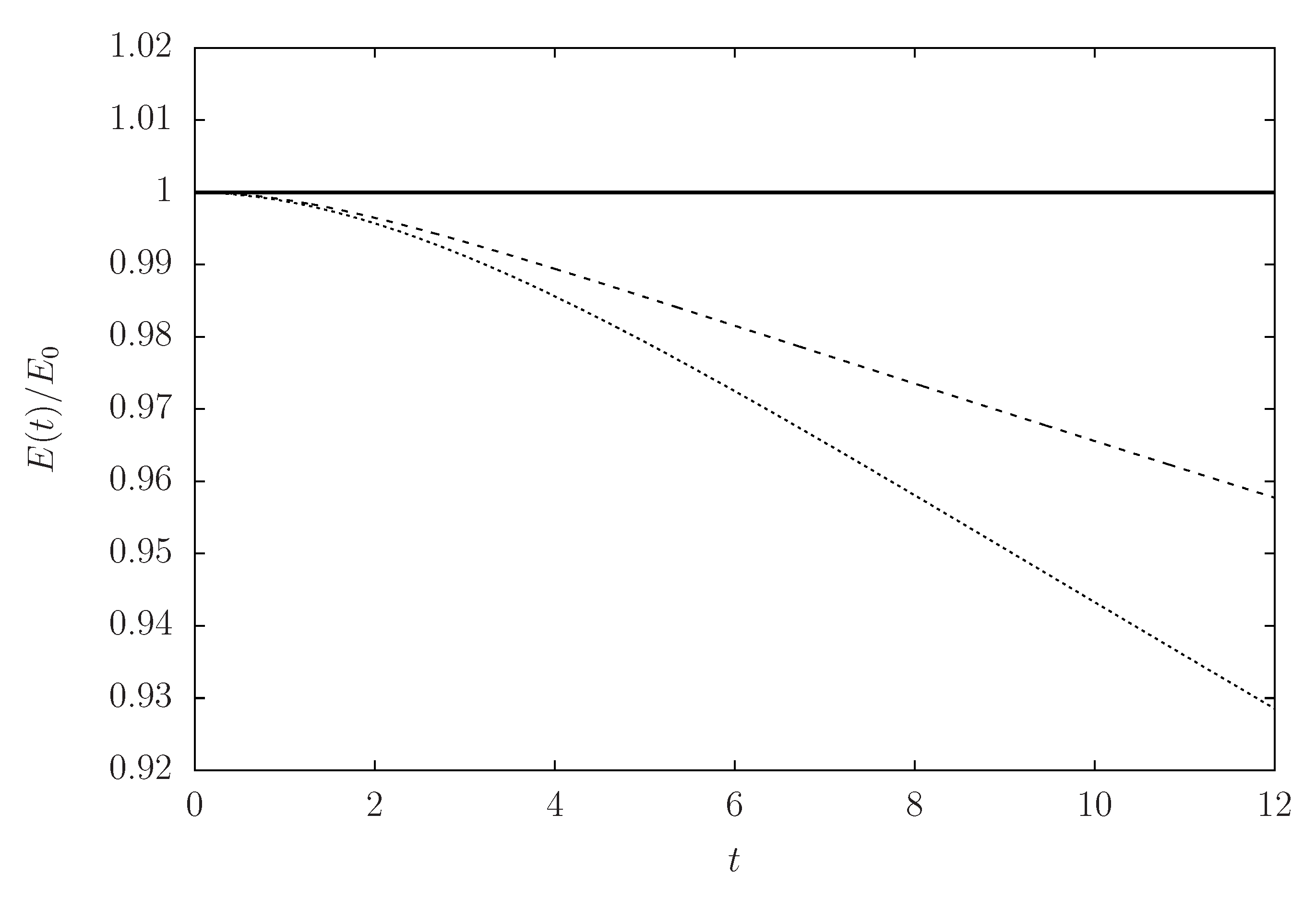
In the inviscid case, it is clear that $E\left(t\right)=E_0=1/4$. The kinetic energy resulting from the numerical integration of the aforementioned solution using PISO and RK4 is shown in Figure 1. Here, a grid of size $32\times 32$ with uniform spacing is used; additionally, a second-order flux interpolation is used for the calculation of the advective term. The RK4 conserves the energy of the system, while pisoFoam exhibits dissipative properties with an error proportional to the time step. From the results shown in Figure 1 is easy to show that the error increases linearly with $∆t$. According to what was previously stated, such error in the PISO algorithm is not due to the relaxation term of Equation (29) neither from the spatial schemes for the different operators used nor to the Rhie–Chow interpolation, since these are also used for RK4. This error originates from the treatment of the advective term, as will be shown next.

The class abstraction for the multiphysics finite-volume framework present in OpenFOAM is thought around the premise of writing hyperbolic PDEs in a natural way, more specifically transport equations. To this end, the following assumption must be made for the time integration of the transport equation of some quantity $\varphi$:

$$\begin{array}{c}\hfill {\left(\frac{\partial u_j\varphi }{\partial x_j}\right)}^{n+1}\approx \frac{\partial u_j^n{\varphi }^{n+1}}{\partial x_j}+O(∆t^{\alpha }),\alpha >1\end{array}$$

Please note that the error induced by this time-splitting depends on the degree of coupling that exists between the velocity and the transported variable $\varphi$. In the case of momentum transport, such splitting introduces an additional approximation, since a Taylor expansion around the time step yields the following

$$\begin{array}{c}\hfill u_j^{n+1}{u}_i^{n+1}=u_j^n{u}_i^{n+1}+u_j^{n+1}{u}_i^n-u_j^n{u}_i^n+O(∆t^2)\end{array}$$

(36)

Please note that the formulation in OpenFOAM only retains one or two of the three terms shown in the right-hand side of the previous equation, depending on the time scheme selected. Such approximation is remedied by the addition of inner iterations in the corrector cycle of PISO, and overall, the algorithm behaves as being first-order accurate in time. On the other hand, in RK4 this operation is not required, and it makes the algorithm more accurate than pisoFoam.

4.2. Hydrodynamic Instabilities: 2D Tollmien–Schlichting Waves

Two-dimensional disturbances occurring in laminar Poiseuille flow, causing transition to turbulence, may be determined using the Orr-Sommerfeld/Squire equations. Such transition, being the least stable mode of the aforementioned equations, is often called K-type transition. This case is of particular interest in the verification of energy-conserving Navier–Stokes solvers since analytic expressions exist for the energy growth rate

$$log\left(\frac{E\left(t\right)}{E_0}\right)=2\left|\alpha c_i\right|t.$$

Please note that the wave velocity c is a complex number, defined as

$$\begin{array}{c}\hfill c=c_r+c_{i}i=-\frac{\lambda }{i\alpha },\end{array}$$

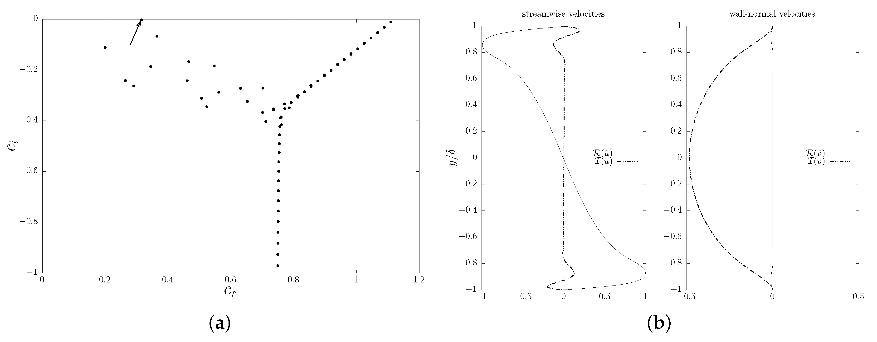
where $\lambda$ is the eigenvalue of the least stable mode for the laminar Poiseuille flows. The least stable mode is then chosen by obtaining the eigenspectrum of the Orr-Sommerfeld equation for a certain critical Reynolds number, $R{e}_{cr}$, based on the centerline velocity, and a streamwise wavelength, $\alpha$. We use the same parameters used by [28], i.e., we use $R{e}_{cr}=5000$ and $\alpha =1.12$ which according to the neutral stability curve for Poiseuille flows, is stable. The resulting eigenspectrum (wave celerities) and eigenvectors for the least stable mode are shown in Figure 2. As a reminder, the velocities $(u,v)$ relate to the eigenvectors $(\widehat{u},\widehat{v})$ in the following way:

$$\begin{array}{c}\hfill u(x,y,t)=\widehat{u}\left(y\right)exp\left[i(\alpha x+\omega t)\right],\\ \hfill v(x,y,t)=\widehat{v}\left(y\right)exp\left[i(\alpha x+\omega t)\right].\end{array}$$

The computational domain is of dimensions $(2\pi /\alpha )\times 2$, and the resolution of the coarsest mesh is $64\times 100$. Notice that due to the linearity and 2-dimensionality of the present initial field, the spanwise direction does not need to be refined nor solved. The perturbation velocities are used as initial fields for the viscous simulation using an amplitude equal to 3% the centerline velocity, in order to guarantee linearity of the solution for the first few iterations.

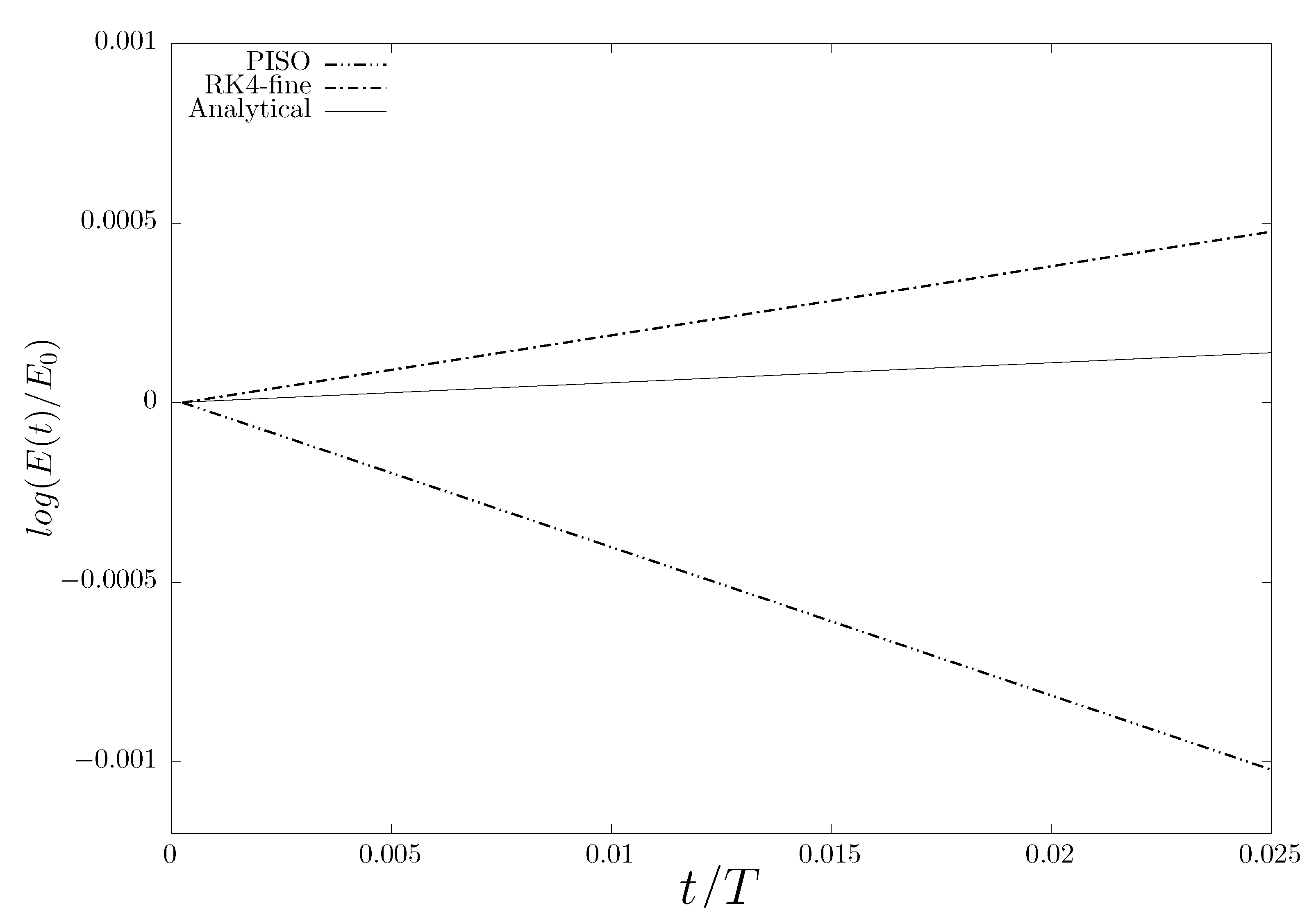
As a reference the energy growth rate for the first few seconds of the simulation is shown in Figure 3, where time is normalized by $T=2\pi /\left(\alpha {\lambda }_r\right)$. Notice that the present method over-predicts the energy growth, situation common when using 4th-order spatial stencils [28], whereas PISO predicts a decay, meaning that the algorithm behaves as simulating a smaller value of $Re$ which does not lie on a stability curve.

An order-of-accuracy analysis is made for which two additional grids are constructed by just doubling the vertical resolution of the previous one. The rate of error reduction can be calculated as

$$\begin{array}{c}\hfill plog\left(2\right)=log\left(\frac{{\varphi }_{\mathit{medium}}-{\varphi }_{\mathit{coarse}}}{{\varphi }_{\mathit{fine}}-{\varphi }_{\mathit{medium}}}\right),\end{array}$$

where $\varphi$ represents a value over which the error is to be calculated, and p the order of error reduction. For the RK4 solver, using the data shown in

Table 1. Computed energy growth at $t/T=0.025$.

Mesh Refinement	$\mathit{E}(\mathit{t}/\mathit{T}=0.025)\times {10}^{-5}$
coarse	1.4945492
medium	1.4947583
fine	1.4948110

, a value of $p\approx 2$ is obtained. The reduction order in this case corresponds to the second-order interpolation used for the discretization of the advective operator. Please note that the error-reduction analysis is made only for the RK4 algorithm, since for PISO it would not make sense in this case.

5. LES of Turbulent Flows

In this Section we report results for LES of two classical turbulent problems. First we consider the canonical plane turbulent channel flow, where the two algorithms are validated for the case of neutral stratification. Successively, we study the Rayleigh–Bènard convection between two horizontal plates.

RK4 is used with the Dynamic Lagrangian Mixed Model (DLMM) already described, while the simulations with PISO use the Dynamic ‘Mean’ Model (DMM) available in OpenFOAM. Note that in both cases we employ the non-uniform Laplacian filter described in Equation (26). Furthermore, for the Rayleigh–Bènard problem, the dynamic evaluation of the sgs scalar fluxes is used except otherwise stated.

Here, the following convention will be used to distinguish between resolved and sgs intensities (or fluctuation) of a certain quantity, $\varphi$,

$$\begin{array}{c}\hfill \varphi (x,y,z,t)=\langle \varphi \rangle (x,y,z)+{\varphi }^{″}(x,y,z,t)+{\varphi }^{\mathit{sgs}}(x,y,z,t),\end{array}$$

where $\langle ·\rangle$ denotes a mean quantity, ${\varphi }^{″}$ are the resolved fluctuations, and ${\varphi }^{\mathit{sgs}}$ are the sgs contributions. Thus, the total fluctuations of $\varphi$ are

$$\begin{array}{c}\hfill {\varphi }^{\prime }(x,y,z,t)={\varphi }^{″}(x,y,z,t)+{\varphi }^{\mathit{sgs}}(x,y,z,t).\end{array}$$

(37)

5.1. LES of Turbulent Poiseuille Flow: Physical Analysis

We consider a turbulent plane channel flow driven by a constant pressure gradient. The frame of reference has x in the streamwise direction, y along the cross-stream direction and z as the wall-normal direction. Here we use the DNS database reported in [29] for a channel flow at $R{e}_{\tau }=\left(u_{\tau }\delta \right)/\nu =800$, where the friction velocity is $u_{\tau }=\sqrt{{\tau }_{wall}/{\rho }_0}$, the half height of the channel is $\delta$, and the kinematic viscosity is $\nu$. The grid spacing is uniform in the $x-y$ plane, whereas the grid is stretched along the z-direction to guarantee adequate resolution near the solid walls. A geometric growth function is used in which the first off-the-wall cell centroid is at $∆z^{+}\approx 0.34$. In order to guarantee a minimum of eight grid points within $z^{+}=10$ a stretching ratio of $7\%$ is used, following Komen et al. [17].

A total of seven simulations were run using different grid distributions in the horizontal direction, and different solvers/LES models.

Table 2. Test and control cases for the verification of the proposed methods in turbulent channel flows.

Case	Grid Dimensions	Domain Size	$(\mathsf{\Delta }{\mathit{x}}^{+},\mathsf{\Delta }{\mathit{y}}^{+})$	Solver	LES Model
RK4Mf	$100\times 100\times 60$	$\frac{4}{3}\pi \times \frac{2}{3}\pi \times 2$	$(33.5,16.76)$	RK4	DLMM
PISOMf				PISO	DLMM
PISONMf					DMM
RK4M	$80\times 80\times 60$	$\frac{4}{3}\pi \times \frac{2}{3}\pi \times 2$	$(41.9,20.9)$	RK4	DLMM
PISOM					DLMM
PISONM				PISO	DMM
PISOuDNS					None

summarizes the cases with their respective characteristics. A first set of cases, hereinafter baseline cases (RK4M, PISOM, PISONM, PISOuDNS), use the horizontal grid spacing constraints proposed by Choi and Moin [30], which are commonly used in the literature of wall-bounded turbulence using LES [24,31,32,33]. Notice that an additional control group composed of three fine grid cases (RK4Mf, PISOMf, PISONMf), using the grid spacing constraints of Komen et al. [17], is studied in order to follow the recommendations made by the aforementioned work regarding resolved LES using commercial codes.

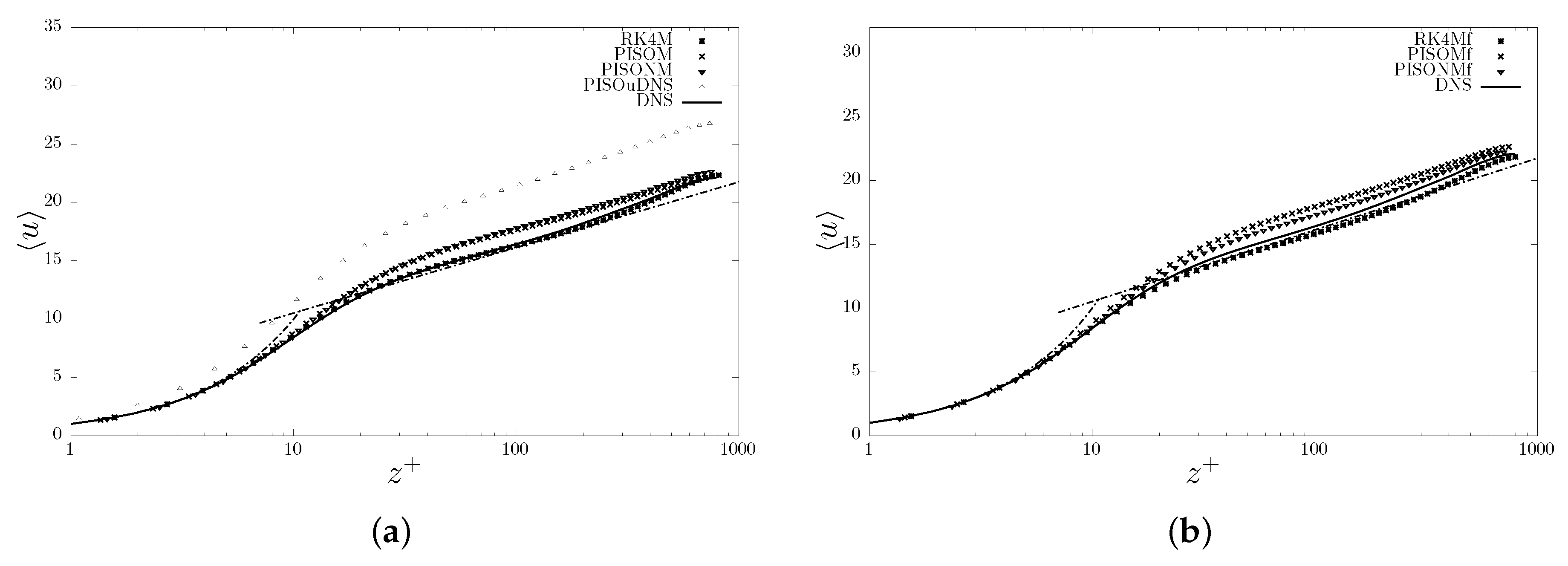
Figure 4 shows the non-dimensional velocity profiles obtained with the two algorithms and different sgs models, together with the uDNS and the DNS reference profiles. The left panel contains data for the baseline grid, the right panel refers to the fine grid. The results obtained using the RK4 algorithm exhibit a very good agreement with reference data; on the other hand, solutions using PISO overestimate the velocity profile, although the results substantially improve with respect to the uDNS. In this kind of simulations, given a constant longitudinal pressure gradient, one obtains the nominal wall shear stress as given by the integral balance of momentum, and a dissipative algorithm overestimates the velocity profile due to an incorrect curvature in the buffer layer. For PISO algorithm, the results show that in the presence of coarser grid, the velocity profile is rather insensitive to the SGS model; on the other hand, when using a finer grid the velocity profile obtained with the eddy-viscosity dynamic model appears somewhat worse than that obtained with the dynamic mixed model.

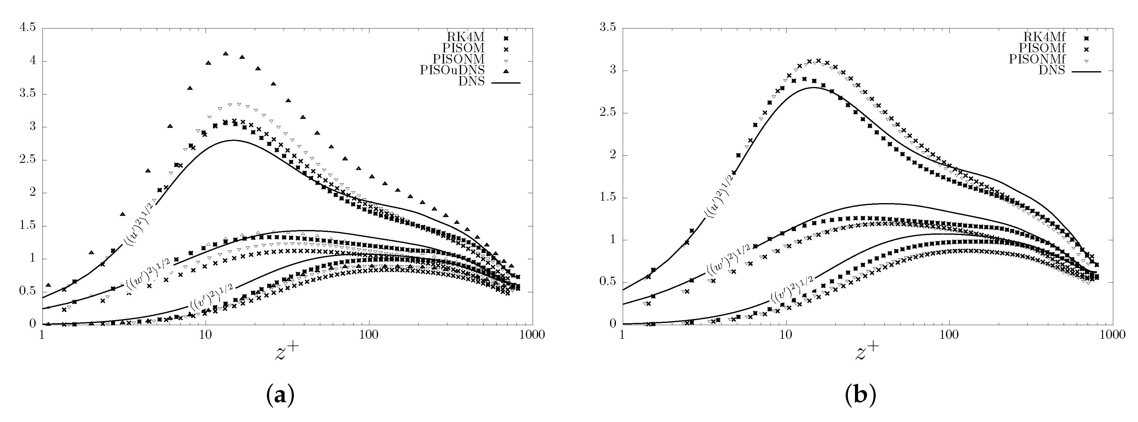
The rms of the diagonal terms of the total (resolved plus SGS) Reynolds stress tensor are shown in Figure 5 for the two grids. The RK4 together with the DLMM gives satisfactory results for the three statistics. PISO exhibits a higher level of fluctuations of the streamwise velocity and smaller level of fluctuations for the other velocity components. Results similar to the ones obtained here are reported also in Komen et al. [17]; in general the over-prediction of the rms of the streamwise velocity component (and under-prediction of the rms of the other components) is due to an abnormal energy redistribution through the pressure-strain correlation of turbulent fluctuations among the three directions. The results are even worse in case of uDNS. Finally, note that the peak of the streamwise component of the Reynolds stresses for the solution obtained with PISO is slightly displaced towards the center of the channel: this may offer a reason for the incorrect resolution of the buffer layer, as previously commented. Overall, the presence of the SGS model in PISO improves the results with respect to the uDNS case, showing that the numerical dissipation does not overwhelm the effect of the model. Also, the dynamic mixed model gives second-order statistics in better agreement when compared with the performance of the dynamic eddy diffusivity model. This is particularly true in the presence of coarse grids.

The mean Reynolds shear stress profiles shown in Figure 6 exhibit behavior within the ranges expected for LESs of channel flow. No particularity can be drawn between the results obtained with PISO using the turbulence model, except for a slight underestimation of ${\tau }_{xz}$ in the outer region of the flow for PISO with LES model. This justifies the mismatch in the mean velocity profile due to the fact that the molecular part of the shear stress appears slightly overestimated by PISO. Furthermore, the uDNS Reynolds stress may give the impression of attaining results similar to DNS but, from the velocity profiles it is clear that such results corresponds to an artificially lower $R{e}_{\tau }$. Once again, the SGS model in the PISO algorithm improves the quality of the results compared to an under-resolved (or equivalently ILES) solution. As for the second-order statistics, the baseline cases using the DLMM seem more accurate than the results obtained with DMM; on the other hand, results obtained for the fine grid cases using DLMM are more accurate, specially for RK4. To be mentioned that the authors have run also simulations using RK4 and the DMM (not shown), obtaining similar results to those obtained with PISO and the DMM.

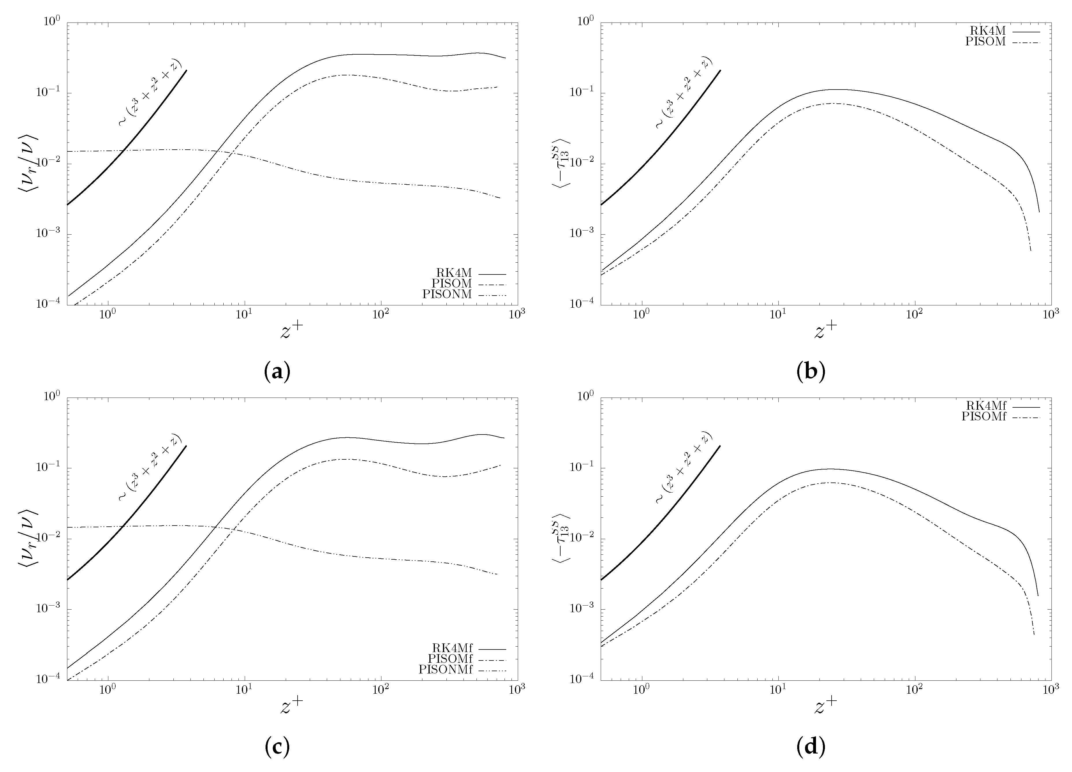
With the aim to analyze the behavior of the filters/LES models herein employed, we carried out an additional analysis which gives an estimation of the growth of the residual eddy viscosity and of the scale-similar shear stress close to the wall. Considering that

$$\begin{array}{cc}\hfill u(x,y,z,t)& =a(x,y,t)z,\hfill \end{array}$$

(38)

$$\begin{array}{cc}\hfill v(x,y,z,t)& =b(x,y,t)z,\hfill \end{array}$$

(39)

$$\begin{array}{cc}\hfill w(x,y,z,t)& =c(x,y,t)z^2,\hfill \end{array}$$

(40)

If one filters the $u-w$ components of the velocity fields using Equation (26), the following relations are obtained:

$$\begin{array}{cc}\hfill \overline{u}& =\overline{a}z+\frac{a}{12}\left(\frac{\partial {∆}_z}{\partial z}\right),\hfill \\ \hfill \overline{w}& =\overline{c}{z}^2+\frac{c}{12}\left(\frac{\partial {∆}_z}{\partial z}z+{∆}_z\right).\hfill \end{array}$$

Now, if one takes the definition of the residual stress component ${\tau }_{13}^r$ as

$$\begin{array}{c}\hfill {\tau }_{13}^r=\overline{uw}-\overline{u}\overline{w},\end{array}$$

(41)

The terms on the RHS are written as:

$$\begin{array}{cc}\hfill \overline{uw}& =\overline{ac}{z}^3+\frac{3ac}{24}\left(\frac{\partial {∆}_z}{\partial z}{z}^2+2{∆}_{z}z\right),\hfill \\ \hfill \overline{u}\overline{w}& =\frac{1}{{12}^2}\left(a\frac{\partial {∆}_z}{\partial z}+12\overline{a}z\right)\left(c{∆}_z+c\frac{\partial {∆}_z}{\partial z}z+12\overline{c}{z}^2\right).\hfill \end{array}$$

From the same empirical relations expressed in Equations (38)–(40) it can be shown that in the vicinity of the wall [34]:

$$\begin{array}{c}\hfill {\tau }_{13}^r=2{\nu }_r{\overline{S}}_{13}\sim 2{\nu }_r\overline{a},\end{array}$$

(42)

Meaning that

$$\begin{array}{c}\hfill \frac{{\nu }_r}{\nu }\sim O(z^3+z^2+z).\end{array}$$

(43)

The same scaling applies for the scale-similar SGS shear stress. Notice that the previous relation holds for the filter herein used; the relation may change if different filters are used, whether filtering is made only along certain directions, or whether the filtering is made in physical space (for a more complete discussion see [35]). For instance, the top-hat filter when used following the approach proposed by Jordan [36] for finite-difference/volume methods leads to the relation

$$\begin{array}{c}\hfill \frac{{\nu }_r}{\nu }\sim O\left(z^3\right).\end{array}$$

The near-wall scaling profiles of the residual viscosity as well of the scale-similar shear stress are shown in Figure 7. Please note that both the eddy diffusivity and the scale-similar contribution are in good agreement with the scaling estimate presented in Equation (43), for the DLMM algorithm proposed in the present work. The normalized turbulent viscosity profiles obtained for the DMM algorithm do not match the scaling estimates presented earlier, and seems to remain roughly constant across the channel. Notice that the sgs contribution of the DMM is about two orders of magnitude less compared to the contributions obtained with DLMM in the logarithmic region.

5.2. LES of Rayleigh–Benard Convection

In this section, we analyze the performance of the two algorithms in a problem of wide interest in the scientific community, namely Rayleigh–Benard Convection (RBC). In canonical RBC the fluid is confined between two horizontal plates, the lower of which is hotter than the upper one. The Rayleigh number rules the intensity of buoyancy with respect to momentum and heat diffusion

$$Ra=\frac{U_f^2{H}^2}{\nu \kappa }=\frac{g\alpha ∆T{H}^3}{\nu \kappa }$$

where $\alpha$ is the thermal expansion coefficient, $∆T$ is the imposed temperature difference between lower and upper plate and H is the gap between the plates; $\kappa$ is the thermal diffusivity of the fluid and $U_f=\sqrt{g\alpha ∆TH}$ the free-fall velocity of a fluid parcel. Other parameters ruling convective processes are the Prandtl number $Pr=\nu /\kappa$ and the aspect ratio of the cell $\mathsf{\Gamma }=L/H$ where L is the horizontal length scale of the domain. In the atmosphere, the convective motions [37] can be very energetic, with values of the Rayleigh number of the order of ${10}^{18}$. Physical experiments with Rayleigh numbers close to that of the atmosphere have been carried out by [38]. Numerical experiments of RBC are typically carried out using Direct Numerical Simulation (DNS) or by LES. The former can afford low-to-moderate values of Rayleigh number, the latter can push the limit of Ra to larger values. LES of RBC in cubic cavities have been performed by [39] and by [40] in the presence of grooves.

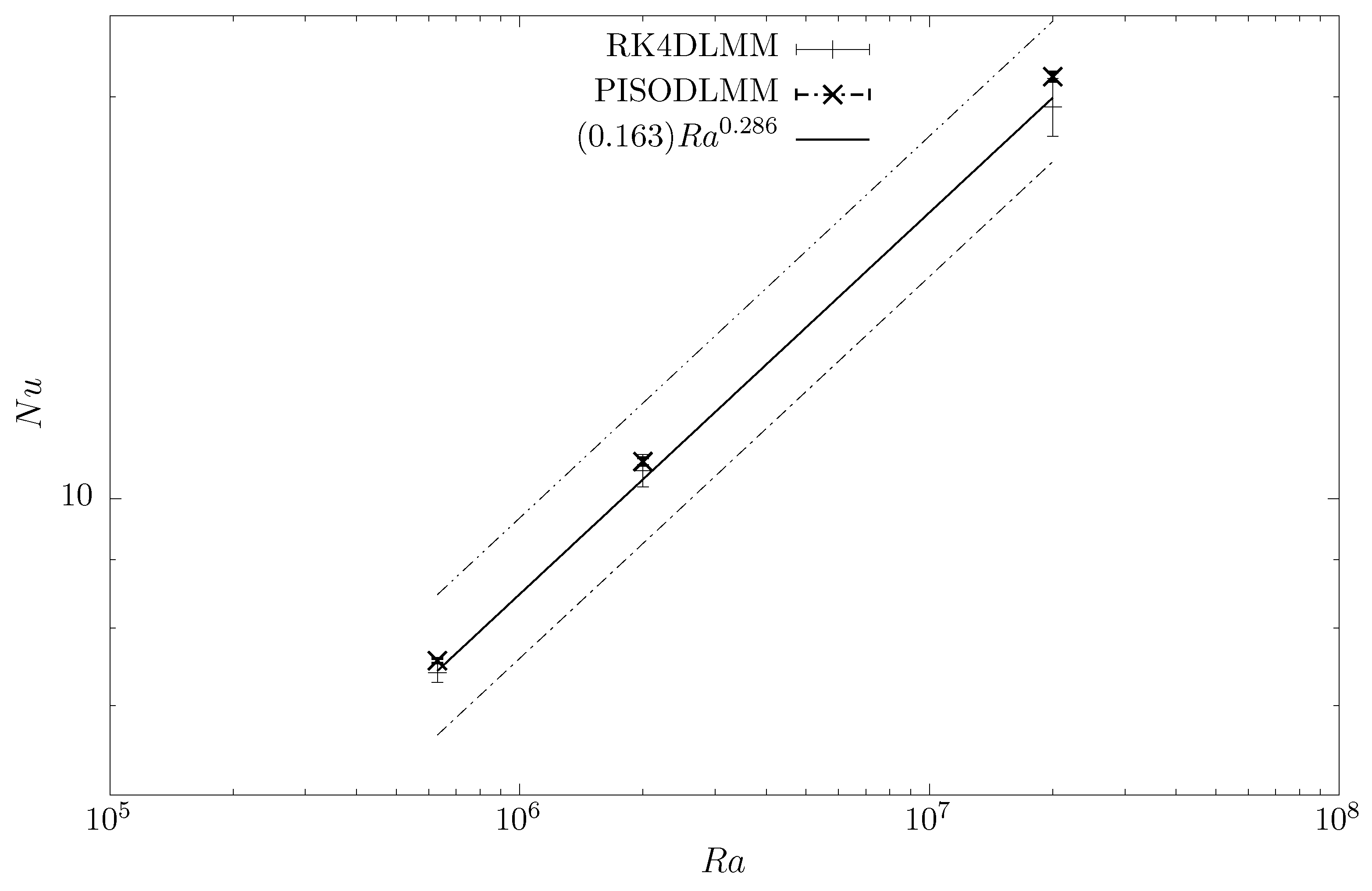
Here, particular attention is paid the study of the relation between $Ra$, a measure of the forcing acting on the flow, and $Nu$ which is a measure of the heat exchange properties of the flow. Such relation may be expressed in the form

$$\begin{array}{c}\hfill Nu=\gamma {Ra}^{\beta }.\end{array}$$

(44)

Such power law is not universal [41]: the $\gamma ,\beta$ coefficients may be function of other non-dimensional parameters. Universality may be assumed in cases where the aspect ratio is unimportant (namely infinite plates), the Rayleigh Number is not very large ($<{10}^{11}$), and for Prandtl numbers larger than $>0.4$. Comparisons with power laws calibrated via DNS [42] and physical experiments [43] will be made, in order to test the performance of the algorithms discussed in the present paper.

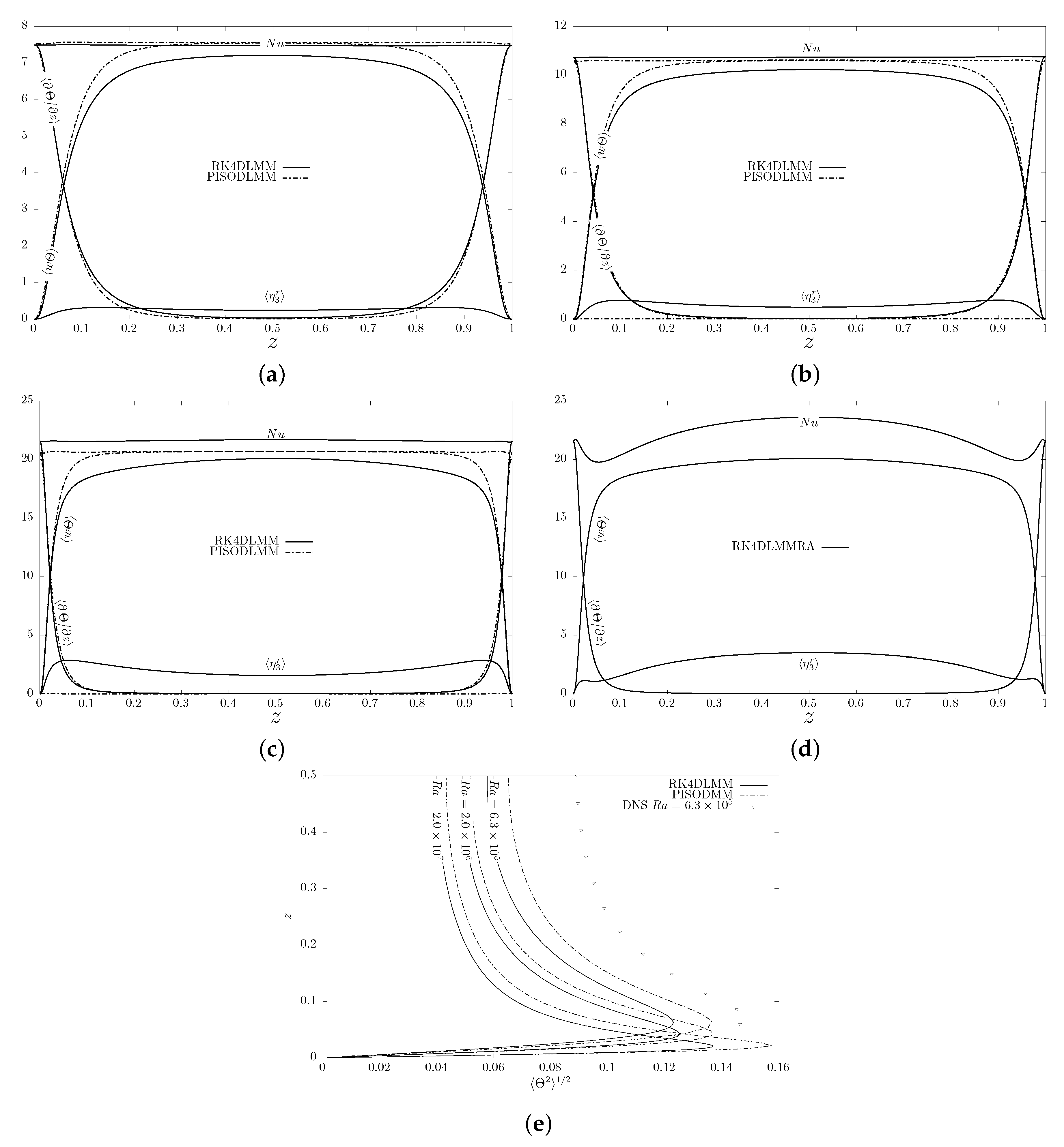
Here we study turbulent convection between two infinite horizontal plates, so that the aspect ratio of the domain is not a free parameter of the problem. The computational domain is $L_x=L_y=6H,L_z=H$ and the grid is composed of $307,200$ hexahedral cells. The spacing along the horizontal directions is set constant, while the mesh is stretched along the vertical direction, in order to adequately reproduce the thermal boundary layer, ${\delta }_{\theta }$. Following the meshing strategy proposed by Verzicco and Camussi [41], at least 6 grid points have been placed within the thermal boundary layer defined as ${\delta }_{\theta }\simeq H/2Nu$. Notice that for $Pr\le 1$, the Kolmogorov scale, $\eta$, is lower or equal to the Batchelor length scale, ${\eta }_T$, but for the $Pr=1$ herein considered these can be regarded as equal. This implies that for wall-resolving LES, the meshing criteria may be based on an accurate resolution of the thermal boundary layer, for which estimates are readily available. The distribution of the grid points is made using the hyperbolic tangent function, clustering them near the plates. The first cell node off the wall is located at $∆z/H=0.001$, which is much smaller than ${\delta }_{\theta }/H\sim 1/2Nu=0.025$ for the largest Rayleigh number herein examined ($Ra=2\times {10}^7$). Periodic boundary conditions are imposed on the horizontal direction (to mimic infinite plates) and no-slip condition on the plates. A summary of the different settings used for the simulations ran in this section are presented in

Table 3. Test cases for the verification of the proposed methods in Rayleigh Bernard Convection.

Case	Grid Dimensions	Domain Size	$(\mathsf{\Delta }\mathit{x},\mathsf{\Delta }\mathit{y},\mathsf{\Delta }{\mathit{z}}_{\mathbf{min}})$	Solver	LES Model
RK4DLMM	$80\times 80\times 48$	$6\times 6\times 1$	$(0.075,0.075,0.001)$	RK4	DLMM
PISODLMM	$80\times 80\times 48$	$6\times 6\times 1$	$(0.075,0.075,0.001)$	PISO	DLMM
RK4DLMMRA	$80\times 80\times 48$	$6\times 6\times 1$	$(0.075,0.075,0.001)$	RK4	DLMM + RA

. The results of three different Rayleigh numbers are analyzed $Ra=6.3\times {10}^5$, $2\times {10}^6$, $2\times {10}^7$. For the sake of clarity, normalization of the wall-normal coordinate, temperature and velocity are made in the following way:

$$\begin{array}{cc}\hfill \mathsf{\Theta }& =\frac{T-T_{\mathit{cold}}}{∆T},\hfill \\ \hfill (u,v,w)& =(u_1,u_2,u_3)/U_f,\hfill \\ \hfill z& =x_3/H,\hfill \end{array}$$

where $T_{\mathit{cold}}$ refers to the temperature in the cold plate, and $U_f$ the free-fall velocity. A first level of analysis of the results obtained using the proposed algorithms can be made by calculating $Nu$ along the vertical. The integral relation

$$\begin{array}{cc}\hfill Nu& =\sqrt{\frac{Ra}{Pr}}\langle w\mathsf{\Theta }+{\eta }_z^c\rangle -\frac{\partial \langle \mathsf{\Theta }\rangle }{\partial z}\hfill \end{array}$$

(45)

Dictates that the Nusselt number must remain constant along the vertical. Please note that the above relation considers the SGS scalar fluxes product of the LES formulation used.

Vertical profiles for each of the terms just discussed, for the $Ra$ considered in this work, are plotted in Figure 8a–c. These results for $Nu$ lie between the ranges calculated using different empirical relations, obtained either by physical or numerical experiments, proposed in the literature [42,43]. Additionally, Figure 8d show the results obtained running the DLMM for momentum and using the RA for the scalar. Near-wall predictions of the Nusselt number are similar to the other simulations, although predictions in the core of the channel show higher SGS fluctuations than expected leading to a non-constant Nusselt profile. The latter results will not be discussed further.

A second level of analysis involves the calculation of the temperature rms profiles. As shown in Figure 8e, the resolved rms profiles are underestimated compared to the DNS results of [44] for the lowest of $Ra$. This is not surprising since the SGS temperature fluctuations are not present in the statistical quantity. The  trend of temperature fluctuations seems to physically represent the thinning of the temperature boundary layer as $Ra$ increases. In general, the solutions obtained with PISO exhibit a higher state of temperature fluctuations, as expected for over-dissipative algorithms.

For an accurate estimation of the $\gamma ,\beta$ parameters of the function $Nu=f\left(Ra\right)$, several other ways of calculating $Nu$ are proposed in the literature:

$$\begin{array}{cc}\hfill Nu& =1+\sqrt{RaPr}{\langle ϵ\rangle }_{\mathit{eff}},\hfill \end{array}$$

(46)

$$\begin{array}{cc}\hfill Nu& =\sqrt{RaPr}\langle N\rangle ,\hfill \end{array}$$

(47)

$$\begin{array}{cc}\hfill Nu& ={\left.\frac{\partial \langle \mathsf{\Theta }\rangle }{\partial z}\right|}_{wall}\hfill \end{array}$$

(48)

where ${\langle ϵ\rangle }_{\mathit{eff}}$ is the effective averaged energy dissipation rate (sgs contributions included), and $\langle N\rangle$ the resolved averaged temperature variance dissipation rate. By volume-averaging each of the quantities just presented at every iteration, one may obtain for each $Ra$ a distribution of $Nu$ in time. The sampling, and time-averaging, is performed over a period of $300H/U_f$, starting from a fully developed flow field.

Results obtained both with pisoFoam and RK4, each using its corresponding turbulence models, is shown in Figure 9. The results obtained using RK4 with the Lagrangian mixed model show increasing variability in the calculation of $Nu$ as $Ra$ increases, whereas for PISO using the Reynolds Analogy such variability is not as strong as it can also be seen in

Table 4. Nusselt number as a function of the Rayleigh number for the results obtained using PISO and RK4, in which the error is taken as the time standard deviation.

$\mathit{Ra}$	$\mathit{Nu}\pm {\langle {\mathit{\sigma }}^2\rangle }^{1/2}$
	PISO	RK4
$6.3\times {10}^5$	$7.561356\pm 0.029477$	$7.4051439417\pm 0.1218679281$
$2.0\times {10}^6$	$10.660694\pm 0.071748$	$10.4987945729\pm 0.2913541913$
$2.0\times {10}^7$	$20.700736\pm 0.168435$	$19.6569584688\pm 0.9787957580$

. A least-square fit, considering the variance of $Ra$, for the RK4 data gives a slope $\beta$ which is very similar to experiments, and the theoretical value ${\beta }_t=2/7$. On the other hand the slope $\beta$ for PISO is slightly higher, indicating the presence of a small amount of ‘artificial’ heat exchange caused by the overall model. However, the rather strong variability shown for the highest $Ra$ using the different approaches for $Nu$ is expected in this case, given the relative under-resolution of the mesh in the horizontal directions.

Typically, the Reynolds Analogy considers that mixing of temperature occurs at the same rate as mixing of momentum, namely that the turbulent Prantdl number $P{r}_r={\nu }_r/{\kappa }_r\sim O\left(1\right)$. This assumption is made explicit by the relation

$$\begin{array}{c}\hfill P{r}_{SGS}={\nu }_{SGS}/{\kappa }_{SGS}=1,\end{array}$$

In the context of LES modeling. Nevertheless, the work of [21], and literature therein cited, shows that this quantity is not constant along the vertical.

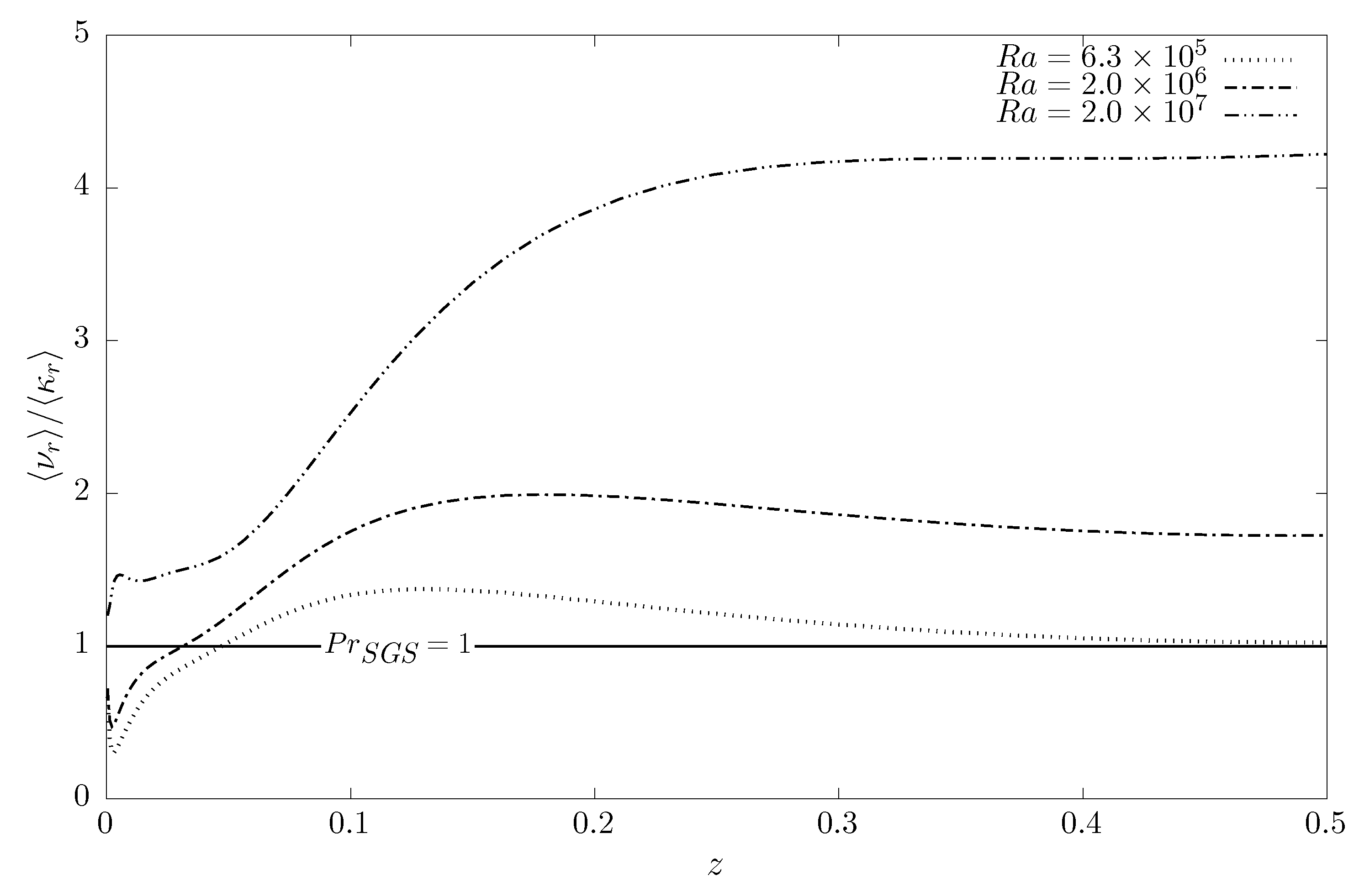
The SGS Prandtl number for the three RBC flows obtained using the present algorithms is shown in Figure 10. Please note that as the $Ra$ increases, the  $P{r}_{SGS}$ increases in the core region. Nevertheless, such ratio does not remain constant across the channel height, and its variation is not monotonic. In the core of the channel, as $Ra$ increases, SGS turbulent momentum mixing tends to be higher than its scalar counterpart. Such scenario may explain the trend of the PISO predictions shown in Figure 10: the assumption $P{r}_{SGS}=1$ under-predicts scalar turbulent mixing for the core portion of the channel, as $Ra$ increases.

6. Conclusions

In the present paper, we compare two different solution methods for the time integration of the Boussinesq form of the NSE, namely the RK4 and PISO. The  PISO along with the DMM algorithms are present within the OpenFOAM library, whereas the RK4 and the DLMM models shown in this work are not.

We first consider the standard implementation of the algorithms in the framework and study the conservation properties using literature test cases, namely the two-dimensional unsteady Taylor vortex and the growth of the linear disturbance in a plane Pouseuille flow under critical conditions. Results of these tests reveal the superiority of the RK4 algorithm over pisoFoam, since the former predicts better the time evolution of the non-linear term in both cases, whereas the latter exhibits dissipative features which may have negative consequences in the study of transitional flows.

Successively, we test the two algorithms within the Smagorinsky LES philosophy: the Dynamic Lagrangian Mixed Model (DLMM), on the other hand the Dynamic ‘Mean’ Model present in OpenFOAM/foam-extend. Also, in case of buoyant flows, the SGS Prandtl number is either evaluated dynamically by the DLMM, or just by setting $P{r}_{SGS}$ constant. The studies involving the DLMM and DMM use the anisotropic Laplace filter.

The use of the RK4 algorithm in conjunction with the DLMM for momentum turbulence show better results compared to those obtained using pisoFoam along with DMM. RK4 together with the DLMM provides good first- and second-order statistics for the neutral wall-bounded flow whereas the results obtained with pisoFoam, although reasonable, are less accurate. This has been attributed both the dissipative character of pisoFoam and to the particularities in the SGS models present in the distributions of OpenFOAM. Interestingly, the use of the SGS model substantially improves the performance of pisoFoam, compared to corresponding coarse DNS (or equivalently ILES) solutions, regardless the LES model. This means that although PISO being more dissipative than RK4, numerical dissipation is not able to overwhelm the effect of the SGS model, and this is probably the feature which has made the algorithm successful in the scientific and engineering communities.

In case of buoyant flows, the Nusselt number predicted using RK4 behaves somewhat better than pisoFoam, although it exhibits some deviations when calculated using different methods. Such deviation is the result of taking into account quantities for which no SGS model is implemented (i.e., the temperature variance.) The analysis of the behavior of the SGS Prandtl number, calculated dynamically within the RK4 LES methodology shows that it tends to 1 in the core region. This clearly shows that the assumption of constant SGS Pr number may produce higher inaccuracies as the $Ra$ number increases, as the cases studied here have shown.

Overall, although pisoFoam exhibits some dissipative features, our tests show that a consistent SGS model is able to improve the results when compared to under-resolved DNS and, as such, it can be still considered a reasonable good algorithm for LES studies. It is robust and provides good results even in the presence of unstructured non-hexahedral meshes, needed when studying very complex geometrical configuration. The RK4 algorithm appears more accurate because of its energy-conserving properties, but its own efficiency in the presence of very stable stratification or in the presence of non-hexahedral meshes has still to be verified. Also, an accurate and robust filter function to be used for non-hexahedral meshes is needed. These issues will be analyzed in upcoming research.

References

- Chorin, A.J. Numerical Solution of the Navier-Stokes Equations. Math. Comp. 1968, 23, 341–362. [Google Scholar] [CrossRef]
- Temam, R. Une methode d’approximation de la solution des equations de Navier-Stokes. Bull. Soc. Math. Fr. 1968, 96, 115–152. [Google Scholar] [CrossRef]
- Kim, J.; Moin, P. Application of a fractional-step method to incompressible Navier-Stokes equations. J. Comput. Phys. 1985, 59, 308–323. [Google Scholar] [CrossRef]
- Le, H.; Moin, P. An improvement of fractional step methods for the incompressible Navier-Stokes equations. J. Comput. Phys. 1991, 92, 369–379. [Google Scholar] [CrossRef]
- Zang, Y.; Street, R.L.; Koseff, J.R. A non-staggered Grid, fractional step method for time-dependent incompressible Navier-Stokes equations in Curvilinear Coordinates. J. Comp. Phys. 1994, 114, 18–33. [Google Scholar] [CrossRef]
- Zang, Y.; Street, R.L.; Koseff, J.R. A dynamic mixed subgrid-scale model and its application to turbulent recirculating flows. Phys. Fluids A Fluid Dyn. 1993, 5, 3186–3196. [Google Scholar] [CrossRef]
- Armenio, V. Large Eddy Simulation in Hydraulic Engineering: Examples of Laboratory-Scale Numerical Experiments. J. Hyd. Eng. 2017, 143. [Google Scholar] [CrossRef]
- Mahesh, K.; Constantinescu, G.; Moin, P. A numerical method for large-eddy simulation in complex geometries. J. Comput. Phys. 2004, 197, 215–240. [Google Scholar] [CrossRef]
- Issa, R.I. Solution of the implicitly discretised fluid flow equations by operator-splitting. J. Comput. Phys. 1986, 62, 40–65. [Google Scholar] [CrossRef]
- Jasak, H. Error Analysis and Estimation for the Finite Volume Method with Applications to Fluid Flows. Ph.D. Thesis, University of London, London, UK, 1996. [Google Scholar]
- Chen, G.; Xiong, Q.; Morris, P.J.; Paterson, E.G.; Sergeev, A.; Wang, Y. OpenFOAM for computational fluid dynamics. Not. AMS 2014, 61, 354–363. [Google Scholar] [CrossRef]
- Weller, H.G.; Tabor, G.; Jasak, H.; Fureby, C. A tensorial approach to computational continuum mechanics using object-oriented techniques. Comput. Phys. 1998, 12, 620–631. [Google Scholar] [CrossRef]
- Grinstein, F.F.; Margolin, L.G.; Rider, W.J. Implicit Large Eddy Simulation: Computing Turbulent Fluid Dynamics; Cambridge University Press: Cambridge, UK, 2007. [Google Scholar]
- Lysenko, D.A.; Ertesvåg, I.S.; Rian, K.E. Large-eddy simulation of the flow over a circular cylinder at Reynolds number 3900 using the OpenFOAM toolbox. Flow Turbul. Combust. 2012, 89, 491–518. [Google Scholar] [CrossRef]
- Vuorinen, V.; Keskinen, J.P.; Duwig, C.; Boersma, B. On the implementation of low-dissipative Runge–Kutta projection methods for time dependent flows using OpenFOAM®. Comput. Fluids 2014, 93, 153–163. [Google Scholar] [CrossRef]
- D’Alessandro, V.; Binci, L.; Montelpare, S.; Ricci, R. On the development of OpenFOAM solvers based on explicit and implicit high-order Runge–Kutta schemes for incompressible flows with heat transfer. Comput. Phys. Commun. 2018, 222, 14–30. [Google Scholar] [CrossRef]
- Komen, E.; Camilo, L.; Shams, A.; Geurts, B.J.; Koren, B. A quantification method for numerical dissipation in quasi-DNS and under-resolved DNS, and effects of numerical dissipation in quasi-DNS and under-resolved DNS of turbulent channel flows. J. Comput. Phys. 2017, 345, 565–595. [Google Scholar] [CrossRef]
- Tuković, Ž.; Perić, M.; Jasak, H. Consistent second-order time-accurate non-iterative PISO-algorithm. Comput. Fluids 2018, 166, 78–85. [Google Scholar] [CrossRef]
- Meneveau, C.; Lund, T.S.; Cabot, W.H. A Lagrangian dynamic subgrid-scale model of turbulence. J. Fluid Mech. 1996, 319, 353–385. [Google Scholar] [CrossRef] [Green Version]
- Vreman, B.; Geurts, B.; Kuerten, H. On the formulation of the dynamic mixed subgrid-scale model. Phys. Fluids 1994, 6, 4057–4059. [Google Scholar] [CrossRef]
- Armenio, V.; Sarkar, S. An Investigation of stably stratified flows using large-eddy simulation. J. Fluid Mech. 2002, 459, 1–42. [Google Scholar] [CrossRef]
- Vasilyev, O.V.; Lund, T.S.; Moin, P. A general class of commutative filters for LES in complex geometries. J. Comput. Phys. 1998, 146, 82–104. [Google Scholar] [CrossRef]
- Germano, M. Turbulence: The filtering approach. J. Fluid Mech. 1992, 238, 325–336. [Google Scholar] [CrossRef]
- Germano, M.; Piomelli, U.; Moin, P.; Cabot, W.H. A dynamic subgrid-scale eddy viscosity model. Phys. Fluids A Fluid Dyn. 1991, 3, 1760–1765. [Google Scholar] [CrossRef]
- Rhie, C.; Chow, W.L. Numerical study of the turbulent flow past an airfoil with trailing edge separation. AIAA J. 1983, 21, 1525–1532. [Google Scholar] [CrossRef]
- Guermond, J.L.; Minev, P.; Shen, J. An overview of projection methods for incompressible flows. Comput. Methods Appl. Mech. Eng. 2006, 195, 6011–6045. [Google Scholar] [CrossRef] [Green Version]
- Gresho, P.M.; Sani, R.L. On Pressure boundary conditions for the incompressible Navier-Stokes Equations. Intl. J. Num. Meth. Fluid 1987, 7, 1111–1145. [Google Scholar] [CrossRef]
- Kaltenbach, H.J.; Driller, D. Phase-error reduction in large-eddy simulation using a compact scheme. In Advances in LES of Complex Flows; Springer: Berlin/Heidelberg, Germany, 2002; pp. 83–98. [Google Scholar]
- Tanahashi, M.; Kang, S.J.; Miyamoto, T.; Shiokawa, S.; Miyauchi, T. Scaling law of fine scale eddies in turbulent channel flows up to Reτ = 800. Int. J. Heat Fluid Flow 2004, 25, 331–340. [Google Scholar] [CrossRef]
- Choi, H.; Moin, P. Grid-point requirements for large eddy simulation: Chapman’s estimates revisited. Phys. Fluids 2012, 24, 011702. [Google Scholar] [CrossRef]
- Rasam, A.; Brethouwer, G.; Schlatter, P.; Li, Q.; Johansson, A.V. Effects of modelling, resolution and anisotropy of subgrid-scales on large eddy simulations of channel flow. J. Turbul. 2011, 12, N10. [Google Scholar] [CrossRef]
- Armenio, V.; Piomelli, U. A Lagrangian Mixed Subgrid-Scale Model in Generalized Coordinates. Flow Turbul. Combust. 2000, 65, 51–81. [Google Scholar] [CrossRef]
- Chong, M.S.; Monty, J.P.; Marusic, I. The topology of surface of surface skin friction and vorticity fields in wall-bounded flows. J. Turbul. 2011, 13, N6. [Google Scholar] [CrossRef]
- Pope, S.B. Turbulent Flows; Cambridge University Press: Cambridge, UK, 2000. [Google Scholar]
- Piomelli, U. High Reynolds number calculations using the dynamic subgrid-scale stress model. Phys. Fluids A Fluid Dyn. 1993, 5, 1484–1490. [Google Scholar] [CrossRef]
- Jordan, S.A. A large-eddy simulation methodology in generalized curvilinear coordinates. J. Comput. Phys. 1999, 148, 322–340. [Google Scholar] [CrossRef]
- Chillà, F.; Schumacher, J. New perspectives in turbulent Rayleigh-Bénard convection. Eur. Phys. J. E 2012, 35, 58. [Google Scholar] [CrossRef] [PubMed]
- Niemela, J.; Skrbek, L.; Sreenivasan, K.; Donnelly, R. Turbulent convection at very high Rayleigh numbers. Nature 2000, 404, 837. [Google Scholar] [CrossRef] [PubMed]
- Foroozani, N.; Niemela, J.J.; Armenio, V.; Sreenivasan, K.R. Influence of container shape on scaling of turbulent fluctuations in convection. Phys. Rev. E 2014, 90, 063003. [Google Scholar] [CrossRef] [PubMed]
- Foroozani, N.; Niemela, J.; Armenio, V.; Sreenivasan, K. Turbulent convection and large scale circulation in a cube with rough horizontal surfaces. Phys. Rev. E 2019, 99, 033116. [Google Scholar] [CrossRef] [PubMed]
- Verzicco, R.; Camussi, R. Numerical experiments on strongly turbulent thermal convection in a slender cylindrical cell. J. Fluid Mech. 2003, 477, 19–49. [Google Scholar] [CrossRef]
- Kerr, R.M. Rayleigh number scaling in numerical convection. J. Fluid Mech. 1996, 310, 139–179. [Google Scholar] [CrossRef]
- Wu, X.Z.; Libchaber, A. Scaling relations in thermal turbulence: The aspect-ratio dependence. Phys. Rev. A 1992, 45, 842. [Google Scholar] [CrossRef] [PubMed]
- Kimmel, S.J.; Domaradzki, J.A. Large eddy simulations of Rayleigh–Bénard convection using subgrid scale estimation model. Phys. Fluids 2000, 12, 169–184. [Google Scholar] [CrossRef]
Figure 1.
Normalized volume-averaged kinetic energy for the inviscid two-dimensional Taylor vortex: Solid line, RK4 with Cou = 0.8; dashed line, pisoFoam with Cou = 0.2; dotted line, pisoFoam with Cou = 0.8.
Figure 2.
(a) Eigenspectrum of the Orr-Sommerfeld/Squire equations for a 2D TS wave of and . The arrow indicates its least stable wave celerity ; (b) streamwise (left) and vertical (right) velocity perturbation coefficients for the least stable mode.
Figure 3.
Energy growth rate obtained for the finest grid using RK4, and for PISO.
Figure 4.
Mean velocity profile scaled using the friction velocity as a function of the distance from the wall in wall units. The dash-dot line represents the log-law profile and the viscous boundary layer velocity profile . (a) Baseline cases; (b) control, or fine grid, cases.
Figure 5.
Total root-mean-square profiles of the velocity components made non-dimensional with the friction velocity. (a) Baseline cases; (b) control, or fine grid, cases.
Figure 6.
Total and residual (SGS) Reynolds shear stress profiles. (a) Baseline cases; (b) control, or fine grid, cases.
Figure 7.
(a,c) Mean SGS viscosity profile normalized by the molecular viscosity; (b,d) Mean scale-similar contribution to the residual Reynolds stress.
Figure 8.
Vertical profiles of the Nusselt number, , the viscous heat flux contribution , the turbulent contribution , and the sgs contributions for: (a) ; (b) ; (c) ; and (d) using the Reynolds Analogy; using RK4 and pisoFoam; Additionally, the (e) temperature RMS for the considered are presented.
Figure 9.
Nusselt number as a function of the Rayleigh number for the results obtained using PISO and RK4. Please note that the results obtained are presented with their corresponding error-bars, taken as one standard deviation of the distributions obtained using different definitions. Line-dots: From [43]; Line-double dots: From [42].
Figure 10.
Profiles of calculated using the present RK4 LES model for the scalar.