Open-Source MASW Inversion Tool Aimed at Shear Wave Velocity Profiling for Soil Site Explorations


1
Faculty of Civil and Environmental Engineering, University of Iceland, Hjardarhagi 2-6, IS-107 Reykjavik, Iceland
2
Pavement Technology, Swedish National Road and Transport Research Institute, SE-581 95 Linköping, Sweden
*
Author to whom correspondence should be addressed.
Geosciences 2020, 10(8), 322; https://doi.org/10.3390/geosciences10080322
Submission received: 12 July 2020
/
Revised: 7 August 2020
/
Accepted: 12 August 2020
/
Published: 17 August 2020
Abstract
:The shear wave velocity profile is of primary interest for geological characterization of soil sites and elucidation of near-surface structures. Multichannel Analysis of Surface Waves (MASW) is a seismic exploration method for determination of near-surface shear wave velocity profiles by analyzing Rayleigh wave propagation over a wide range of wavelengths. The inverse problem faced during the application of MASW involves finding one or more layered soil models whose theoretical dispersion curves match the observed dispersion characteristics. A set of open-source MATLAB-based tools for acquiring and analyzing MASW field data, MASWaves, has been under development in recent years. In this paper, a new tool, using an efficient Monte Carlo search technique, is introduced to conduct the inversion analysis in order to provide the shear wave velocity profile. The performance and applicability of the inversion scheme is demonstrated with synthetic datasets and field data acquired at a well-characterized geotechnical research site.
1. Introduction
Shear wave velocity () is a fundamental parameter in geological engineering due to its relations to the small-strain shear stiffness (). Various techniques exist for evaluation of in-situ -profiles [1,2,3], including both invasive techniques and active- and passive-source surface wave analysis methods. Information on the shear wave velocity distribution is essential for assessing the dynamic behavior of soil, e.g., for analysis of seismic site response, soil-structure interaction, and vibration transmission in soils [4,5,6]. Current building codes use the average shear wave velocity in the top-most 30 m () as a proxy to classify soil sites and account for the effects of the local soil conditions on the seismic action [7,8]. is also commonly implemented in ground motion prediction equations to consider expected soil amplifications [9,10,11]. Recently proposed classification schemes have further suggested the use of the average shear wave velocity over the top-most meters (), alongside other geotechnical parameters, for seismic zonation purposes (e.g., [12,13,14,15]). Other emerging applications of active- and passive-source measurements of include assessments of the depth to bedrock or engineering bedrock [16,17,18], and detection of fault zones [19]. Surface wave analysis has also been proposed as a monitoring tool, where repeated measurements are carried out to assess the quality and depth of soil improvement or compaction [20,21]. The shear wave velocity of soil materials has further been related to numerous other geotechnical parameters through empirical correlations (e.g., [4,22,23,24,25]).
The dispersive nature of Rayleigh waves in a heterogeneous medium provides key information for characterization of near-surface materials [4] and subsequent elucidation of subsurface structures. At a given site, the -profile has a dominant effect on the Rayleigh wave dispersion. Multichannel Analysis of Surface Waves (MASW) [26] is a non-invasive method that has become a common technique for estimating near-surface -profiles for engineering applications [27,28,29]. MASW is a time- and cost-effective technique. It can further be applied at a wide variety of soil sites, including locations where site conditions limit the application of invasive techniques, such as penetration tests [30,31]. An application of MASW can be divided into three consecutive steps: (i) field measurements, (ii) identification of experimental dispersion curves, and (iii) inversion for shear wave velocity. The present paper addresses the inverse problem faced in the third step of the analysis.
In brief, the inversion entails iteratively comparing theoretical dispersion curves, obtained from ‘trial’ layered subsurface models, to the experimental data in search of a model that both fits the observed dispersion characteristics and incorporates known features of the survey site. Overall, the resolution of surface wave analysis methods diminishes with depth [1]; while the analysis can resolve modest variations in shear wave velocity and layering close to the surface, only major variations can be detected at greater depths. A common practice for interpretation of fundamental mode dispersion curves (e.g., [2,26,29,32]) is to estimate the investigated depth as one-third to half the longest retrieved wavelength (), and, similarly, to limit the thickness of the top-most layer to one-third to half the shortest wavelength. Recently, alternatives to this empirical wavelength-depth approach have been proposed [33,34,35,36], such as directly transforming the wavelength of the experimental dispersion curve to the depth of a corresponding pseudo -profile. The layering parameterization is further an important factor in the inversion process [32,37] and the number of layers to include in a stratified soil model should be regarded as an additional inversion parameter. However, no general recommendations exist for how to optimally specify the number of soil layers, although repeated inversion using different parameterizations has been recommended [29,32].
An open-source MATLAB-based software, MASWaves (version 1.0, University of Iceland, Reykjavík, Iceland), has been developed for acquiring, processing, and inverting active-source MASW registrations [38] (see also masw.hi.is). The previous implementation of the MASW analysis uses trial-and-error iteration during the inversion process, whilst an automated inversion procedure is preferred. In general, such automated techniques can be divided into local and global search procedures [27,39]. Local search methods are iterative schemes which, by starting from an initial estimate of the inversion parameters, generate a sequence of improved model assessments. Global search methods, however, attempt to search for the global stationary point by exploring the entire solution space. Use of various advanced optimization methods has been suggested to guide the search towards the high-probability-density regions of the solution space (e.g., [40,41,42,43,44,45,46,47,48]). An inherent risk associated with local search methods is that the algorithm may converge to a local minimum of the misfit function. Inaccurate values of the partial derivatives of the dispersion curve with respect to the model parameters can also severely affect the performance of the algorithm. Despite these drawbacks, local search methods may be preferred by engineers as they are easier to handle than advanced global search procedures. They further provide the result in the form of a single -profile, which is desirable for many engineering applications [27]. Global search procedures avoid the assumption of linearity between the experimental data and the model parameters. However, they are, in general, computationally more demanding as a high number of forward simulations is required to adequately sample the model parameter space [27], thereby imposing some practical limitations on the analysis. While global search methods are better suited for the non-uniqueness of the inverse problem encountered, using highly complex optimization algorithms in order to conduct the analysis within a reasonable time frame might be considered a disadvantage for geological engineering applications in practice.
In this paper, a new open-source inversion tool is introduced as a part of the MASWaves software. The objective of this work was to explore the use of an efficient Monte Carlo-based global search procedure that only requires the implementation of a simple random sampling scheme but can deliver reliable soil stiffness profiles. The applied methodology is described. The applicability and performance of the new module is then demonstrated; first, by analysis of synthetic dispersion curves, representing loose to medium-dense sand and soft clay sites as frequently encountered in practice. The algorithm was further tested on synthetic dispersion curves that were perturbed by introduction of white Gaussian noise. Finally, a dataset, acquired at a well-characterized geo-test site, was analyzed to verify the robustness of the proposed strategy. As recommended by Olafsdottir et al. [49], the dataset includes a statistical sample of dispersion curves which makes it possible to quantify the variability in estimated phase velocity values. After conducting the Monte Carlo-based search, using different layering parameterizations, inference is drawn from the set of simulated -profiles based on the observed spread in the experimental data. The results are compared to invasive measurements of shear wave velocity previously conducted at the site.
2. Method
For forward computation of Rayleigh wave dispersion curves, the survey site is modeled as a linear elastic semi-infinite layered medium consisting of a predefined number () of homogeneous and isotropic layers over a half-space (Figure 1). The layered model is defined in terms of shear wave velocity , compressional wave velocity , density and layer thickness . Alternatively, the Poisson’s ratio can be specified for each layer instead of its compressional wave velocity. The observed experimental dispersion curve is denoted by ().
A schematic overview of the inversion strategy is provided in Figure 2. The shear wave velocity has a dominant effect on the fundamental mode dispersion curve at frequencies higher than 5 Hz, followed by layer thicknesses [50], while variations in other material properties have much less effect [1,51]. Thus, the focus is on inversion of the elements of and . Hence, the number of unknown model parameters (given a fixed value of ) is reduced from to .
The compressional wave velocity (or Poisson’s ratio) and density are estimated based on a-priori information or experience of similar soil types from other sites. Prior studies have indicated that an unreasonable choice of these model parameters may affect the estimated shear wave velocity profiles [29,52,53,54]. Thorough analysis of available information is, therefore, important for assessing the values of (or ) and . A reasonable estimate of the groundwater level is key to conducting the inversion analysis. The velocity of compressional waves propagating through unsaturated soils is governed by the stiffness of the soil skeleton. For soft saturated soils, the compressional waves are propagated by the groundwater and their propagation velocity controlled by the bulk compressibility of the water [1,4]. As dispersion curves associated with unsaturated (i.e., low and low ) and saturated (i.e., low and high ) soil models differ significantly [29], an unreasonable estimate of the groundwater level may lead to substantial errors in the inverted shear wave velocity profile. For assessment of the density profile, values obtained from independent soil investigations are preferred. If such information is not available, it has been recommended to specify a vertical density trend that is consistent with the expected geology, instead of using a constant value of for the entire section [54].
Initial estimates of and are required as a starting point of the inversion process. Other, user-defined, inputs are the search-control parameters and , and the maximum number of iterations . During the inversion process, the parameters and specify the range of shear wave velocity and layer thickness values, respectively, that the algorithm can sample in each iteration. The effects of specifying different values for the search-control parameters (hereafter also referred to as ‘-parameters’) are studied in subsequent sections.
The initial shear wave velocity value for each layer is obtained by mapping the experimental dispersion curve into approximate values of . Subsequently, the pseudo-shear wave velocity profile is discretized to match the previously assumed layer structure following a method comparable to the schemes adopted by Xia et al. [50] and de Lucena and Taioli [51], i.e.,
where the wavelength is estimated as to where is the average depth of the -th layer, i.e., . In the examples presented in the following sections, a value of is used. The multiplication factor in Equation (1) is specified as 1.09 based on the ratio between the propagation velocities of shear and Rayleigh waves in a homogenous medium. The value of can also be estimated for specific soil materials as [55]
where is Poisson’s ratio.
At sites where the observed fundamental mode dispersion curve has vertical asymptotes (e.g., model A in Figure 3), those can be used to improve the estimate of the initial shear wave velocity values [50]. Hence, the asymptotic velocities and are used in Equation (1) for assessment of and . Vertical asymptotes of an experimental dispersion curve can be visually identified by plotting the curve in the phase velocity-wavelength domain. A given experimental dispersion curve is considered to have a vertical asymptote at the shortest retrieved wavelengths () if there exists a vertical line () to which the curve seems to draw arbitrarily close as it recedes to . Likewise, the curve is considered to have a vertical asymptote at the longest retrieved wavelengths () if it approaches a vertical line () as approaches . If the experimental dispersion curve does not show such vertical asymptotes, and can be estimated as and , respectively.
The theoretical Rayleigh wave phase velocities that correspond to each element of are obtained using the initial set of model parameters (i.e., , , (or ) and ). The fast delta-matrix algorithm [56] is used for computation of theoretical dispersion curves. The misfit between the theoretical and experimental dispersion curves is defined as
where and are the Q-dimensional experimental and theoretical phase velocity vectors, respectively. The dispersion misfit is abbreviated as DC misfit in the following discussion.
For changing the shear wave velocity vector in each iteration, a set of numbers (with ) is sampled from the uniform distribution and added to the elements of , i.e.,
where the resulting vector is referred to as the ‘testing shear wave velocity vector’. The layer thickness vector is modified in an analogous way, with a random number () sampled for each of the finite-thickness layers and added to , providing the ‘testing layer thickness vector’ , i.e.,
Hence, the elements of and will vary randomly but will at most differ by % and % from the corresponding elements of and , respectively, in each iteration.
A-priori information on the tested site, as well as inference drawn from the shape of the experimental dispersion curve, can be used to further constrain the inversion to target the high-probability-density regions of the solution space. This includes a normally dispersive parameterization, i.e., an increase in velocity with depth, or predefined ranges for the elements of or within certain depths. Such additional constraints may be implemented by restricting the Monte Carlo (MC) sampling to fulfill the added conditions. Alternatively, the sampling can be conducted as described by Equations (4) and (5) and sets of simulated parameters subsequently accepted or rejected based on the sampling criteria.
The elements of and are updated in each successful iteration (Figure 2). More detailed, the theoretical dispersion curve () is reevaluated using the testing profile defined by , , (or and . If the testing profile provides a better fit to the observed data (i.e., a lower value of the dispersion misfit, Equation (3)) than any previously tested profile, the shear wave velocity and layer thickness vectors are updated as and . Otherwise, the model parameters are not changed. Hence, the search is centered around the ‘best fitting’ shear wave velocity profile that has been obtained at each point during the inversion. This simulation is repeated times.
3. Synthetic Data Inversion
Three synthetic models were used to demonstrate the performance of the inversion scheme. The models represent different situations that may be encountered in near-surface soil site investigations, including both normally dispersive soil profiles and a profile with velocity reversals. Model A (Table 1) depicts a simple two-layer structure. Models B and C (Table 2) represent different multi-layered structures and are based on models used by Tokimatsu et al. [57] to study the dispersion properties of fundamental and higher mode Rayleigh waves in a layered medium. Model B is characterized by a gradual increase in shear wave velocity with depth, whereas in model C, a stiffer layer is sandwiched between two softer layers. The shear wave velocity structure of the synthetic models was designed so that the profiles would represent loose to medium-dense sand sites and soft clay sites [29,58,59]. In each of the three models, the groundwater table is assumed to be located at a great depth.
Figure 3 depicts the fundamental mode dispersion curves corresponding to the three synthetic models. For inversion of the synthetic data, the dispersion curves were sampled at 60 equally spaced points within a wavelength interval of 1–60 m. This range is consistent with what might be expected when conducting active-source measurements at comparable real-world sites.
For inversion of the synthetic dispersion curves, the search-control parameters were specified as = = with . Hence, in each iteration, both the shear wave velocity and layer thickness testing values could deviate up to % from the corresponding parameters of the lowest dispersion misfit model obtained at that point in the inversion process. The density and Poisson’s ratio were fixed at their original values. In each inversion iteration, the elements of were recomputed based on the Poisson’s ratio and the elements of the testing shear wave velocity vector. For models A and B, a normally dispersive parameterization was specified, whereas velocity reversals were permitted within the top 15 m for inversion of the data from model C. The number of iterations in each run of the algorithm (Figure 2) was = 1000. As the search of the optimum -profile is based on a Monte Carlo process, the inversion scheme was initiated ten times (using identical starting models) to reduce the effects of the randomized sampling. Inference was subsequently drawn from the resulting dataset consisting of 10 × 1000 trial -profiles.
Uncertainties associated with the experimental MASW data may arise from a variety of factors. These include spatial variability in subsoil material properties at a given site, measurement and sampling errors (e.g., due to limitations of the measurement equipment or an imprecise measurement profile set-up), and coherent or uncorrelated noise in the recorded signal. It is difficult to quantify how the error associated with the recorded time series is propagated through the different data processing steps [60]. The manual aspect of the dispersion curve identification may further introduce additional uncertainties to the dispersion curve estimates. Nevertheless, it is possible to provide a measure of the error associated with the experimental data by collecting repeated shots and evaluating the statistical distributions of the extracted phase velocity values at each frequency or wavelength [49]. In general, the longer wavelength (lower frequency) part of the dispersion curve has been found to be characterized by higher uncertainty than its shorter wavelength (higher frequency) range [60,61].
In this work, accepted -profiles are defined as the set of profiles whose associated dispersion curves fall within one standard deviation of the average experimental curve. For the interpretation of inversion results for the unperturbed synthetic data, the experimental standard deviation was approximated as a ratio of the true phase velocity at each wavelength, i.e.,
The value of was estimated as 0.05 independent of wavelength. The estimated value is based on experimental values from several sites with a shear wave velocity structure comparable to the synthetic models [61]. It is, however, noted that the uncertainty usually increases with wavelength in real-world scenarios, and values somewhat lower than 0.05 may be expected at short wavelengths.
In addition to presenting the inversion results in terms of interval velocity profiles, they were evaluated in terms of how accurately they recover the true values of as averaged over the top-most meters, defined as
where and denote the shear wave velocity and thickness of the -th layer, respectively, for a total of layers down to depth [7].
3.1. Two-Layer Unperturbed Synthetic Model
The inversion of the unperturbed synthetic data from model A was first conducted by assuming a two-layer geologic structure (i.e., one finite-thickness layer over a half-space) for the testing shear wave velocity profiles and with = 10. For further evaluating the ability of the inversion scheme to recover the true -profile, the inversion was initiated using two different models with the layer interface located at depths of 2 m and 10 m, respectively. The true depth of the layer interface is 4 m (Table 1). The initial shear wave velocity values were determined as described by Equation (1). Figure 4 and Figure 5c illustrate the inversion results. The true shear wave velocity and layer thickness values from Table 1, and the corresponding dispersion curve and -profile, are shown using red dotted lines. Dashed lines indicate the initial models and the associated dispersion curves. The - and - profiles whose dispersion curves deviated less than 5% from the synthetic curve at all wavelengths were sorted based on dispersion misfit values (Equation (3)). The darkest colors indicate the profiles whose dispersion curves best fit the synthetic data. The lowest dispersion misfit - and - profiles resulting from each run of the algorithm (i.e., within each set of = 1000 iterations) are further shown. Note that these profiles are not necessarily the ten profiles whose dispersion curves best fit the target curve within the combined set of 10,000 iterations. For example, the second-lowest dispersion misfit profile resulting from the -th initiation might have a lower dispersion misfit value than the ‘best fitting’ profile (i.e., lowest dispersion misfit model) from the -st initiation. In the case of the two-layer trial models, the lowest DC misfit profiles from each of the ten runs are visually indistinguishable and almost identical to the true profile.
To test a soil model characterized by a very sharp velocity contrast, the half-space velocity of model A was changed to = 800 m/s and the inversion repeated. The altered model represents a case where a thin sedimentary layer sits on top of a stiff layer, that may be classified as seismic bedrock. The analysis delivered inverted -profiles with comparable level of accuracy as obtained for the original model A. That is, the search algorithm was able to identify the depth of the sharp velocity contrast, as well as retrieving the shear wave velocity of both the sedimentary layer and the stiff half-space.
Figure 5 further illustrates the effects of changing the values of the search-control parameters to = 2.5 (Figure 5a), = 5 (Figure 5b) and = 20 (Figure 5d) for inversion of the synthetic dispersion curve for model A (Table 1). The results depicted were obtained by initially placing the layer interface at a depth of 10 m. The simple algorithm managed in all cases to retrieve -profiles that match the synthetic profile, even though the initial estimate of the theoretical dispersion curve corresponded very poorly to the synthetic data. For application of the search algorithm, upper and lower bounds for the search area were not specified. However, the light gray areas in Figure 5, which display all the simulated testing profiles, provide a visual indication of the part of the model parameter space that was sampled. Overall, increasing the value of increases the size of the explored solution space. However, given a fixed number of iterations, an increased value of inevitably leads to more variation within the set of testing -profiles (i.e., more sparse sampling of the parameter space).
Figure 6 shows the effects of the different -values on the data and model fitting progression for each of the cases presented in Figure 5. The data fitting criteria is a measure of how well the theoretical dispersion curves fit the target dispersion curve. It therefore serves as a basis for the best model selection in the MC simulations. Figure 6a illustrates how often, within the set of 10 × 1000 simulations, the search algorithm finds a new set of model parameters with better data fitting (i.e., a lower dispersion misfit value). The model fitting is a measure of how well the sampled sets of model parameters fit the synthetic model, and thus, displays how well the inverted - and -profiles match the underlying true profiles. The model fitting is defined in terms of - and -profile misfit values (Equations (8) and (9)), defined analogously to the dispersion misfit, i.e.,
where and are the true shear wave velocity and layer thickness values of the -th layer and and are the corresponding testing values. The true and trial -profiles are denoted by and , respectively, where is the number of sample points.
To evaluate the effects of over-parameterizing the inversion, the analysis was repeated by assuming testing shear wave velocity profiles with four () and eight layers (including the half-space) and = 10. The initial sets of model parameters were specified such that the layer thicknesses were constant or increased with depth. That is, = [1, 2, 5] m for the model and = [1, 1, 1, 2, 3, 4, 6] m for the model, where denotes the initially specified layer thickness vector. The initial shear wave velocity values were obtained with Equation (1) by using the mid-point of each finite-thickness layer as a reference for evaluation of . The inversion results are presented in Figure 7. In both cases, within the 10 × 1000 iterations, the inversion algorithm converged to theoretical dispersion curves that fit the synthetic data well, as indicated by dispersion misfit values of 0.3% and 0.8%, respectively. The corresponding reconstructed -profiles were further in reasonably good agreement with the true profile and did correctly indicate the existence and location of the sharp layer interface that characterizes the true model. However, as a result of the over-parameterization, there was substantially more variation within the set of accepted -profiles as compared to the results obtained by assuming a two-layer model (see Figure 4 and Figure 5). The same applies to the variability within the set of lowest dispersion misfit - and -profiles obtained with the ten independent initializations.
3.2. Four-Layer Unperturbed Synthetic Models
Model B depicts a normally dispersive soil profile consisting of three finite-thickness layers over a half-space. First, the inversion of the unperturbed synthetic data from model B was conducted by assuming a four-layer geologic structure , where the initially specified layer thicknesses increased with depth (Figure 8). The target dispersion curve for model B (Figure 3) does not display predominant vertical asymptotes. Hence, the initial shear wave velocity values for the surficial layer and the half-space were obtained using the Rayleigh wave velocities corresponding to = 1 m and = 60 m, respectively.
Figure 9 shows the inversion results of the unperturbed synthetic data from model B, as obtained by specifying the search-control parameters as (a) = 2.5, (b) , (c) = 10 and (d) = 20. The - and -profiles whose dispersion curves deviated less than 5% from the synthetic curve at each wavelength are plotted on top of the 10 × 1000 randomly generated testing profiles. The profiles characterized by the lowest dispersion misfit values are indicated by the darkest colors, and the lowest misfit profiles resulting from each run of the algorithm are compared in the rightmost column of Figure 9. The theoretical dispersion curves associated with these ten profiles all adequately match the synthetic data. However, due to the inversion non-uniqueness, there is some variation within the set of profiles, especially for the = 20 case (Figure 9d) and, to lesser extent, the = 10 case (Figure 9c). Nevertheless, the corresponding estimates of for different depths are consistent with their true values.
Analysis of inversely dispersive sites presents a challenge for the application of MASW, both regarding the dispersion analysis and the inversion. For evaluating the behavior of the inversion strategy when subjected to an inversely dispersive target model, the algorithm was tested on the synthetic dispersion curve from model C (Figure 3), where a stiffer layer is trapped between two softer layers. The inversion was conducted using the same initial layering parameterization and the same -parameter values as for inversion of the data from model B. The results are reported in Figure 10 using the same format as in Figure 9. Overall, the inverted -profiles in Figure 10a–c (that were obtained with = 2.5, = 5 and = 10) are consistent with the true profile and retrieve the existence and approximate location of the velocity reversal. However, substantially more variation was observed within the set of reconstructed -profiles in the = 20 case.
Figure 11 and Figure 12 illustrate the effects of the different -values on the data and model fitting progression for each of the cases presented in Figure 9 (model B) and Figure 10 (model C). The data fitting was quantified in terms of the dispersion misfit values, whereas the - and -profile misfits, defined by Equations (8) and (9), were used as measures of the model fitting. The unbroken lines in Figure 11 and Figure 12 indicate the average fitness behavior of the ten independent initializations for each -value. The shaded areas correspond to plus-minus one standard deviation of the average behavior.
To study the effects of under- or over-parameterizing the soil model, the inversion of the unperturbed dispersion curves of models B and C was repeated by assuming testing profiles with 3, 6, 8 and 12 layers (Figure 8). The inversion results are presented in Figure 13 (for model B) and Figure 14 (for model C), using the same format as in Figure 9 and Figure 10. Figure 15 further compares the lowest dispersion misfit -profiles resulting from each tested layering parameterization to the true profiles. Overall, the results indicate that an improper parameterization may deliver a -profile that, despite a low dispersion misfit value, does not correctly represent prominent features of the true model. An assumption of too few layers can result in an overly simplistic -profile that does not adequately describe the variation in material properties with depth. If a parameterization consisting of excessively many layers is assumed, the resulting -profile may be unreasonably complicated. For instance, the inversion results for model B obtained by assuming a 12-layer profile (Figure 13d) fail to detect the prominent increase in at a depth of 14 m. Nevertheless, the general trend of the true -profile for model B was detected in all cases (Figure 15a) and the average shear wave velocity values () were, overall, very consistent with their true values (Figure 13).
By including more than four layers in the testing -profiles for model C, the search algorithm was further able to identify the approximate location and characteristic velocity of the stiffer layer and provide estimates of consistent with their true values (Figure 14 and Figure 15b). However, by severely over-parameterizing the model (Figure 14c), the inversion scheme tended to smooth out prominent changes in in the same way as was observed for model B (Figure 15). Under-parameterizing the assumed model provides insufficient resolution for detection of the higher-velocity layer, leading to insufficient inversion results with the ‘best fitting’ dispersion curve (within the combined set of 10,000 iterations) deviating substantially from the target curve.
3.3. Inversion of Perturbed Synthetic Dispersion Curves
In real-world situations, acquired surface wave records are affected by measurement and sampling errors and coherent or uncorrelated noise in the recorded signal [60,62]. Possible inter-analyst variability during the data analysis is another source of uncertainty. In particular, the visual identification and manual/semi-manual picking of dispersion curves from spectral images can be affected by human bias. As a result, identified experimental dispersion curves are inevitably subjected to error, which can alter the misfit function topography and complicate the inversion process [46,63]. To evaluate the effects of noise on the performance of the inversion scheme, the algorithm was also tested on perturbed data. The synthetic dispersion curves of models A, B and C, respectively, were perturbed by introduction of a 5% white Gaussian noise (Figure 16) and the inverse procedure subsequently applied on the perturbed data. The assumption of Gaussian distribution for variations in phase velocity is consistent with prior studies on related topics [45,46].
The inversion was conducted using identical layering parameterizations as in Figure 5, Figure 9 and Figure 10, for the three models, respectively, i.e., a two-layer structure with the initial location of the layer interface at a depth of 10 m for model A, and the four-layer structure depicted in Figure 8 for models B and C. Figure 17 illustrates the inversion of the perturbed synthetic dispersion curves. The values of the search-control parameters were specified as = 10. The 100 (i.e., 1%) lowest dispersion misfit - and -profiles within each simulated dataset are plotted on top of the 10 × 1000 randomly generated testing profiles in Figure 17b,c (for model A), Figure 17f,g (for model B) and Figure 17j,k (for model C). The profiles whose dispersion curves best fit the corresponding target curve are indicated by the darkest colors. The dispersion curves associated with each trial model are shown using the same color scale in Figure 17a,e,i. The lowest dispersion misfit - and -profiles resulting from each run of the algorithm (i.e., within each set of 1000 iterations) are further shown in Figure 17d,h,l, for models A, B and C, respectively. As shown in Figure 17, the inversion scheme provided in all three cases acceptable - and -profiles that are consistent with the underlying true profiles. Therefore, the results demonstrate the robustness of the inversion scheme in the presence of Gaussian noise.
4. Field Data Inversion
For further evaluation of the inversion scheme, the methodology was tested on data acquired at a Norwegian National Geo-Test Site (NGTS, www.geotestsite.no) in the town of Halden in South Norway [64]. The Halden testing area is approximately 6000 m2 and its topography is relatively flat. The top-most soil unit at the site consists of a 4.5–5 m thick layer of loose to medium-dense silty sand. It rests on a layer of normally consolidated, low plasticity silt that extends down to a depth of around 15–16 m. A unit of low to medium strength clay is found at the bottom of the silt deposit [65,66]. The depth to bedrock within the testing area has been found to increase from its northeastern corner to the southwest. However, in the southern part of the site, where the measurements reported in this section were conducted, bedrock is typically identified at a depth of 21 m [66,67]. Hence, soil layering beneath the measurement profile is considered to reasonably conform to the 1D subsurface model associated with MASW testing (Figure 1). The groundwater table is located at a depth of about 2 m, as measured from an in-situ standpipe [66].
Since 2015, the Halden site has been thoroughly characterized with various geological, geotechnical, and geophysical analysis tools. An overview of the engineering properties and the decomposition of the Halden silt is provided by Blaker et al. [66]. In particular, its shear wave velocity distribution was evaluated in a series of Seismic Cone Penetration Tests (SCPT) and Seismic Dilatometer Marchetti Tests (SDMT) that were carried out as a part of the NGTS project [64,65,67]. Results from SCPT and SDMT surveys that were conducted in close vicinity to the MASW profile were used for comparison purposes in this work.
The MASW measurements were conducted by using 24 vertical geophones (GS-11D from Geospace Technologies, Houston, TX) with a natural frequency of 4.5 Hz and a critical damping ratio of 0.5. The geophones were arranged in a linear array with an equal receiver spacing of 1 m and connected to two data acquisition cards (NI USB-6218 from National Instruments, Austin, TX) and a laptop computer equipped with a customized data acquisition software. The impact load was created by a sledgehammer that was struck on a 15 cm-diameter metallic base plate at a 3 m and 5 m distance, respectively, from each end of the receiver spread. Repeated shots were recorded for each source location to obtain a statistical sample of dispersion curves and allow for quantification of the variability in the estimated phase velocity values. Due to geological constraints, i.e., the decreasing depth to bedrock towards northeast, the use of a receiver spread longer than 23 m was not considered reasonable. Examples of the experimental data are presented in Figure 18a (forward shot) and Figure 18b (reverse shot). The recording time for each shot was 2.0 s with a sampling frequency of 1000 Hz and a pre-trigger duration of 0.2 s. However, for display purposes, only the first 0.9 s of each recorded trace are shown in Figure 18a,b. The corresponding dispersion images are shown in Figure 18c,d.
The dispersion analysis tool of MASWaves [38] was used for processing the acquired time series and identifying the fundamental mode of Rayleigh wave propagation. The fundamental mode dispersion curve estimates that were identified from the repeated shots, are compared in Figure 18e. The experimental dispersion curves obtained by using different source offset lengths were in good agreement, as indicated by a coefficient of variation below 5% at each frequency (Figure 18f). In line with previous findings [49,60], the lowest frequency components displayed more variability than components in the higher frequency range. Analysis of shots applied at both ends of the receiver spread further indicated comparable fundamental mode dispersion characteristics and therefore not implying the presence of significant lateral variations in material properties below the receiver spread. Prior to the inversion, experimental dispersion curve estimates from repeated shots were added up within logarithmically (i.e., log3) spaced wavelength intervals following the procedure described by Olafsdottir et al. [49], resulting in a composite experimental dispersion curve over the wavelength range of 2–32 m.
The inversion was conducted without using the known layer structure of the site to guide the layering parameterization. This was done to mimic the common situation encountered in near-surface geological investigations, where only limited information about the layering of the test area is available. Hence, the number of finite-thickness layers () was handled as an unknown parameter and the inversion conducted using eight different parameterizations consisting of two to nine layers (including the half-space). Velocity reversals were permitted within the testing shear wave velocity profiles down to a depth of approximately 10 m. The density profile was specified based on results of independent soil investigations previously conducted at the site [65,66]. The compressional wave velocity was fixed at = 1440 m/s below the groundwater level. The Poisson’s ratio of the unsaturated soil layer(s) was estimated as 0.35 [68] and the corresponding values recomputed in each iteration based on the elements of the testing shear wave velocity vector. A total of 10 × 1000 testing shear wave velocity profiles was sampled for each layering parameterization. In our experience, the computations (i.e., ten initiations) routinely take approximately 5 min when performed on a standard PC desktop computer (with an Intel i7-8700 processor and 16 GB of RAM).
Overall, the same considerations hold regarding selection of -parameter values as for inversion of the synthetic data (refer to Figure 5, Figure 9 and Figure 10). Particularly, an increased -parameter ( and/or ) value prompts more variability within the set of tested shear wave velocity and layer thickness values, respectively. Hence, given a fixed number of iterations, the somewhat sparser sampling risks inferior fit (i.e., higher dispersion misfit values) between the experimental and theoretical dispersion curves, although the lowest dispersion misfit profiles associated with the different -parameter values may be visually comparable.
Based on results presented in preceding sections, as well as preliminary inversion of the dispersion data from the Halden site, the values of the -parameters were specified as = 5 and = 10. The initial pseudo-shear wave velocity estimates obtained by Equation (1) (indicated by dashed lines in Figure 19) were overall adequately close to their inverted values, prompting the use of a lower . However, as the initially specified layer thicknesses were manually defined, a larger value of was deemed more appropriate to allow for more variation within the set of sampled layer thicknesses. Figure 19 presents results obtained by parameterizing the soil profile as (a) three layers (), (b) four layers (), (c) six layers (), and (d) eight layers (). The theoretical dispersion curves that best fit the observed dispersion characteristics (i.e., fell within one standard deviation of the composite experimental curve at all wavelengths) are illustrated using a color scale. The corresponding - and -profiles are shown using the same colors; also shown are the lowest dispersion misfit profiles resulting from each of the ten initiations. Figure 20b shows the lowest dispersion misfit -profiles obtained from each tested parameterization, whereas the associated theoretical dispersion curves are compared to the experimental data in Figure 20a. The corresponding -profiles are shown in Figure 20c. Figure 21 compares the set of inverted -profiles to results of SDMT and SCPT measurements carried out in close proximity to the MASW profile.
Overall, the results presented in Figure 21b indicate a very good agreement between the MASW and SDMT measurements. The SCPT data are slightly scattered; however, the MASW results are very comparable to the general trend demonstrated by the SCPT (Figure 21a). Apart from the two-layer parametrization, all the theoretical dispersion curves shown in Figure 20a visually match the experimental data and provide dispersion misfit values well below 0.5%. Hence, given a deterministic analysis assuming a fixed layering parameterization, each one of them might be considered an adequate solution. The -profiles associated with the different layering parameterizations (except for the two-layer model) are further nearly identical. However, by increasing the number of layers (refer to Figure 19c,d), even lower dispersion misfit values and smoother velocity interval profiles, that visually seem to agree better with the results of the invasive measurements, were obtained. Hence, a six- or eight-layer parametrization may be considered more appropriate for the site.
5. Discussion
The objective of the inversion analysis is to obtain a -model that realistically represents the characteristics of the test site. The inverse problem faced in MASW analysis is by nature ill-posed, non-linear, mix-determined and non-unique. That is, multiple significantly different -profiles can provide theoretical dispersion curves that match the experimental data similarly well in terms of dispersion misfit values [1,32]. Hence, available information about the test area should be used to constrain the inversion and aid the selection of realistic models.
Discrete parameterization of the survey site is a crucial starting point of the inversion process. In the absence of relevant a-priori information, the analyst must blindly assess the number of layers to be included in the trial models. Conducting the inversion by using several different parameterizations has been strongly encouraged in previous studies [e.g., 29,32]. The findings of this work further support the necessity of implementing the number of finite-thickness layers () as an additional inversion parameter and conduct repeated analyses to assess the effects of the model parameterization.
The strategy adopted here was to start the analysis with a small number of layers (i.e., ). Subsequently, the number of layers included in the trial models was increased and the inversion process repeated. Due to the mix-determined nature of the inverse problem, the layer thicknesses were specified such that they were constant or increased with depth. The thickness of the top-most soil layer and the depth to the half-space top were further specified such that they fulfilled the general recommendations associated with the empirical wavelength-depth approach. Based on our experience, the number of different parameterizations that may need to be tested is highly site-specific. Commonly, a value of in the range of three to seven gives fair results for near-surface soil characterization. If two different parameterizations result in comparable dispersion misfit values and provide -profiles whose dispersion curves visually fit the experimental data equally well over the entire wavelength (or frequency) range, the model consisting of fewer layers is generally chosen by the authors. That is, the objective is to provide sufficient resolution to retrieve variations in close to the surface, while avoiding severe over-parameterization that might lead to an unreliable -profile, due to a lack of data to constrain the inversion. This approach is consistent with the recommendations provided by Foti et al. [29]. However, for applications of MASW where the sole objective is to assess the average shear wave velocity of the site (e.g., ), the results presented here suggest that the layering parameterization plays a minor role, provided that the inversion is not severely under-parameterized and converges to a model whose theoretical dispersion curve is consistent with the experimental data. This is consistent with previous findings (e.g., [3,69,70,71,72]), demonstrating the robustness of surface wave analysis for assessment of .
For applications of the inversion tool, the maximum number of iterations (in each run of the algorithm) was specified as . The search-control parameters and were specified in the range of 2.5 to 20 (i.e., 2.5% to 20%). The results of this study demonstrated that the use of -parameters in the range of 5 to 10 was sufficient in all the cases, i.e., for near-surface applications at loose to medium-dense clay, sand or silt sites. Due to the experimental uncertainties associated with both the data acquisition and the dispersion analysis, the values of the dispersion misfit function may not be comparable between different sites. Therefore, it is not recommended to specify a global misfit-threshold to stop the iteration process. Instead, the search algorithm completes a fixed number of generations. Subsequently, inference is drawn from the set of simulated -profiles based on the observed spread in the experimental data. Using = 1000 and 10 initiations (10 × 1000) gave fair results for engineering purposes in all the cases in this study. Allowing the algorithm to continue for more than 1000 iterations (in each run) might, in some cases, have provided even lower dispersion misfit values. However, as observed dispersion curves are, to some extent, affected by coherent and uncorrelated noise, extremely low dispersion misfit values may not be realistic [73].
6. Conclusions
The dispersive properties of Rayleigh waves propagating through a heterogeneous medium provide key information about the elastic properties of the subsurface materials. This paper presents an efficient Monte Carlo-based global search scheme for solving the inverse problem of identifying realistic -profiles from experimental Rayleigh wave dispersion curves. The inversion scheme is incorporated in a revised version of the MASWaves software, a set of open-source MATLAB-based tools for acquiring, processing, and analyzing MASW field data. The software can be downloaded, along with sample data and user guidelines, at masw.hi.is.
The performance and applicability of the inversion algorithm is demonstrated using both synthetic datasets, representing loose to medium-dense sand and soft clay sites commonly encountered in practice, and field data acquired at a well-characterized research site. Overall, the inversion results for the synthetic datasets indicate that the algorithm can be successfully used for inversion of fundamental mode Rayleigh wave dispersion curves. The analysis of the real-world data further verifies the performance of the inversion scheme. The obtained shear wave velocity estimates match those obtained with invasive techniques. Hence, these findings indicate that a simple global search technique, i.e., not incorporating any advanced optimization, can effectively deliver reliable stiffness profile estimates for engineering applications.
The inverse problem associated with MASW surveys is inherently non-unique. Hence, interpretation of surface wave data requires subjective judgment and fully automatic search processes are complicated to implement. The results of this study support the recommendation of conducting a preliminary analysis using multiple different parameterizations. Taking into consideration any a-priori information about the test site and the shape and wavelength range covered by the observed dispersion curve is further important to aid the selection of realistic models. In addition, presenting the inversion results as a set of layered soil models whose theoretical dispersion curves fit the observed data (e.g., fall within one standard deviation of the experimental curve) provides an indication of the uncertainty associated with the assessments for subsequent applications.
Author Contributions
Conceptualization, E.A.O., S.E. and B.B.; methodology, E.A.O.; software, E.A.O.; investigation, E.A.O., S.E. and B.B.; formal analysis, E.A.O.; validation, E.A.O., S.E. and B.B.; writing—original draft preparation, E.A.O.; writing—review and editing, E.A.O., S.E. and B.B.; supervision, S.E. and B.B.; funding acquisition, E.A.O., S.E. and B.B. All authors have read and agreed to the published version of the manuscript.
Funding
This research was funded by the Icelandic Research Fund, grant number 206793-051, the University of Iceland Research Fund, grant number 73077, the Icelandic Road and Coastal Administration, grant number 1800-373, and the Energy Research Fund of the National Power Company of Iceland, grant number NYR-18-2017.
Acknowledgments
The authors would like to thank the organizers of the NGTS project (www.geotestsite.no) for assistance prior to and during the in-situ measurements at the Halden research site, as well as for providing access to results of geotechnical and geophysical measurements conducted at the site.
Conflicts of Interest
The authors declare no conflict of interest. The funders had no role in the design of the study; in the collection, analyses, or interpretation of data; in the writing of the manuscript, nor in the decision to publish the results.
References
- Foti, S.; Lai, C.G.; Rix, G.J.; Strobbia, C. Surface Wave Methods for Near-Surface Site Characterization; CRC Press, Taylor & Francis Group: Boca Raton, FL, USA, 2015; pp. 3–36. [Google Scholar]
- Garofalo, F.; Foti, S.; Hollender, F.; Bard, P.-Y.; Cornou, C.; Cox, B.R.; Ohrnberger, M.; Sicilia, D.; Asten, M.; Di Giulio, G.; et al. InterPACIFIC project: Comparison of invasive and non-invasive methods for seismic site characterization. Part I: Intra-comparison of surface wave methods. Soil Dyn. Earthq. Eng. 2016, 82, 222–240. [Google Scholar] [CrossRef] [Green Version]
- Garofalo, F.; Foti, S.; Hollender, F.; Bard, P.-Y.; Cornou, C.; Cox, B.R.; Dechamp, A.; Ohrnberger, M.; Perron, V.; Sicilia, D.; et al. InterPACIFIC project: Comparison of invasive and non-invasive methods for seismic site characterization. Part II: Inter-comparison between surface-wave and borehole methods. Soil. Dyn. Earthq. Eng. 2016, 82, 241–254. [Google Scholar] [CrossRef] [Green Version]
- Kramer, S.L. Geotechnical Earthquake Engineering; Pearson Educated Ltd.: Harlow, Essex, UK, 2014; pp. 184–419. [Google Scholar]
- Towhata, I. Geotechnical Earthquake Engineering, 1st ed.; Springer: Berlin/Heidelberg, Germany, 2008; pp. 87–119, 149–179. [Google Scholar]
- Wolf, J.P. Dynamic Soil-Structure Interaction; Prentice-Hall, Inc.: Englewood Cliffs, NJ, USA, 1985; pp. 1–12. [Google Scholar]
- CEN. EN1998-1:2004. Eurocode 8: Design of Structures for Earthquake Resistance. Part 1: General Rules, Seismic Actions and Rules for Buildings; European Committee for Standardization (CEN): Brussels, Belgium, 2004. [Google Scholar]
- BSSC. NEHRP (National Earthquake Hazards Reduction Program) Recommended Seismic Provisions for New Buildings and Other Structures (FEMA P-1050-1) 2015 Edition. Vol. 1. Part 1: Provisions. Part 2: Commentary; Federal Emergency Management Agency: Washington, DC, USA, 2015.
- Abrahamson, N.; Atkinson, G.; Boore, D.; Bozorgnia, Y.; Campbell, K.; Chiou, B.; Idriss, I.M.; Silva, W.; Youngs, R. Comparisons of the NGA ground-motion relations. Earthq. Spectra. 2008, 24, 45–66. [Google Scholar] [CrossRef] [Green Version]
- Douglas, J.; Aochi, H. A survey of techniques for predicting earthquake ground motions for engineering purposes. Surv. Geophys. 2008, 29, 187–220. [Google Scholar] [CrossRef] [Green Version]
- Douglas, J.; Edwards, B. Recent and future developments in earthquake ground motion estimation. Earth-Sci. Rev. 2016, 160, 203–219. [Google Scholar] [CrossRef] [Green Version]
- Héloïse, C.; Bard, P.-Y.; Duval, A.-M.; Bertrand, E. Site effect assessment using KiK-net data: Part 2—site amplification prediction equation based on f0 and VSZ. Bull. Earthq. Eng. 2012, 10, 451–489. [Google Scholar] [CrossRef]
- Luzi, L.; Puglia, R.; Pacor, F.; Gallipoli, M.R.; Bindi, D.; Mucciarelli, M. Proposal for a soil classification based on parameters alternative or complementary to VS,30. Bull. Earthq. Eng. 2011, 9, 1877–1898. [Google Scholar] [CrossRef]
- Pitilakis, K.; Riga, E.; Anastasiadis, A. New code site classification, amplification factors and normalized response spectra based on a worldwide ground-motion database. Bull. Earthq. Eng. 2013, 11, 925–966. [Google Scholar] [CrossRef]
- Pitilakis, K.; Riga, E.; Anastasiadis, A.; Fotopoulou, S.; Karafagka, S. Towards the revision of EC8: Proposal for an alternative site classification scheme and associated intensity dependent spectral amplification factors. Soil Dyn. Earthq. Eng. 2019, 126, 105137. [Google Scholar] [CrossRef]
- Anbazhagan, P.; Sitharam, T.G. Spatial Variability of the Depth of Weathered and Engineering Bedrock using Multichannel Analysis of Surface Wave Method. Pure Appl. Geophys. 2009, 166, 409–428. [Google Scholar] [CrossRef]
- Moon, S.-W.; Hayashi, K.; Ku, T. Estimating Spatial Variations in Bedrock Depth and Weathering Degree in Decomposed Granite from Surface Waves. J. Geotech. Geoenviron. Eng. 2017, 143, 04017020. [Google Scholar] [CrossRef]
- Moon, S.-W.; Subramaniam, P.; Zhang, Y.; Vinoth, G.; Ku, T. Bedrock depth evaluation using microtremor measurement: Empirical guidelines at weathered granite formation in Singapore. J. Appl. Geophys. 2019, 171, 103866. [Google Scholar] [CrossRef]
- Ivanov, J.; Miller, R.D.; Lacombe, P.; Johnson, C.D.; Lane, J.W., Jr. Delineating a shallow fault zone and dipping bedrock strata using multichannal analysis of surface waves with a land streamer. Geophysics 2006, 71, A39–A42. [Google Scholar] [CrossRef] [Green Version]
- Karray, M.; Lefebvre, G.; Ethier, Y.; Bigras, A. Assessment of deep compaction of the Péribonka dam foundation using “modal analysis of surface waves” (MASW). Can. Geotech. J. 2010, 47, 312–326. [Google Scholar] [CrossRef]
- Bitri, A.; Samyn, K.; Brûlé, S.; Javelaud, E.H. Assessment of ground compaction using multi-channel analysis of surface wave data and cone penetration tests. Near Surf. Geophys. 2013, 11, 683–690. [Google Scholar] [CrossRef] [Green Version]
- Hussien, M.N.; Karray, M. Shear wave velocity as a geotechnical parameter: An overview. Can. Geotech. J. 2016, 53, 252–272. [Google Scholar] [CrossRef]
- Moon, S.W.; Ku, T. Empirical estimation of soil unit weight and undrained shear strength from shear wave velocity measurements. In Geotechnical and Geophysical Site Characterisation 5, Proceedings of the Fifth International Conference on Geotechnical and Geophysical Site Characterisation, Gold Coast, Queensland, Australia, 5–9 September 2016; Lehane, B.M., Acosta-Martínez, H.E., Kelly, R., Eds.; Australian Geomechanics Society: Sydney, Australia, 2016; pp. 1247–1252. [Google Scholar]
- L’Heureux, J.-S.; Long, M. Relationship between Shear-Wave Velocity and Geotechnical Parameters for Norwegian Clays. J. Geotech. Geoenviron. Eng. 2017, 143, 04017013. [Google Scholar] [CrossRef] [Green Version]
- Wair, B.R.; DeJong, J.T.; Shantz, T. Guidelines for Estimation of Shear Wave Velocity Profiles. PEER Report 2012/08; Pacific Earthquake Engineering Research Center: Davis, CA, USA, 2012.
- Park, C.B.; Miller, R.D.; Xia, J. Multichannel analysis of surface waves. Geophysics 1999, 64, 800–808. [Google Scholar] [CrossRef] [Green Version]
- Socco, L.V.; Foti, S.; Boiero, D. Surface-wave analysis for building near-surface velocity models–Established approaches and new perspectives. Geophysics 2010, 75, 75A83–75A102. [Google Scholar] [CrossRef]
- Xia, J. Estimation of near-surface shear-wave velocities and quality factors using multichannel analysis of surface-wave methods. J. Appl. Geophys. 2014, 103, 140–151. [Google Scholar] [CrossRef]
- Foti, S.; Hollender, F.; Garofalo, F.; Albarello, D.; Asten, M.; Bard, P.-Y.; Comina, C.; Cornou, C.; Cox, B.; Di Giulio, G.; et al. Guidelines for the good practice of surface wave analysis: A product of the InterPACIFIC project. Bull. Earthq. Eng. 2018, 16, 2367–2420. [Google Scholar] [CrossRef]
- Bessason, B.; Erlingsson, S. Shear wave velocity in surface sediments. Jökull 2011, 61, 51–64. [Google Scholar]
- Olafsdottir, E.A.; Bessason, B.; Erlingsson, S. Application of MASW in the South Iceland Seismic Zone. In Geotechnical, Geological and Earthquake Engineering, Vol. 47. Proceedings of the International Conference on Earthquake Engineering and Structural Dynamics; Rupakhety, R., Olafsson, S., Bessason, B., Eds.; Springer: Cham, Switzerland, 2019; pp. 53–66. [Google Scholar]
- Cox, B.R.; Teague, D.P. Layering ratios: A systematic approach to the inversion of surface wave data in the absence of a priori information. Geophys. J. Int. 2016, 207, 422–438. [Google Scholar] [CrossRef] [Green Version]
- Leong, E.C.; Aung, A.M.W. Weighted average velocity forward modelling of Rayleigh surface waves. Soil Dyn. Earthq. Eng. 2012, 43, 218–228. [Google Scholar] [CrossRef]
- Haney, M.M.; Tsai, V.C. Nonperturbational surface-wave inversion: A Dix-type relation for surface waves. Geophysics 2015, 80, EN167–EN177. [Google Scholar] [CrossRef] [Green Version]
- Socco, L.V.; Comina, C.; Khosro Anjom, F. Time-average velocity estimation through surface-wave analysis: Part 1–S-wave velocity. Geophysics 2017, 82, U49–U59. [Google Scholar] [CrossRef]
- Passeri, F. Development of An Advanced Geostatistical Model for Shear Wave Velocity Profiles to Manage Uncertainties and Variabilities in Ground Response Analyses. Ph.D. Thesis, Politecnico di Torino, Torino, Italy, 15 March 2019. [Google Scholar]
- Di Giulio, G.; Savvaidis, A.; Ohrnberger, M.; Wathelet, M.; Cornou, C.; Knapmeyer-Endrun, B.; Renalier, F.; Theodoulidis, N.; Bard, P.-Y. Exploring the model space and ranking a best class of models in surface-wave dispersion inversion: Application at European strong-motion sites. Geophysics 2012, 77, B147–B166. [Google Scholar] [CrossRef] [Green Version]
- Olafsdottir, E.A.; Erlingsson, S.; Bessason, B. Tool for analysis of multichannel analysis of surface waves (MASW) field data and evaluation of shear wave velocity profiles of soils. Can. Geotech. J. 2018, 55, 217–233. [Google Scholar] [CrossRef] [Green Version]
- Sen, M.K.; Stoffa, P.L. Global Optimization Methods in Geophysical Inversion, 2nd ed.; Cambridge University Press: Cambridge, UK, 2013; pp. 29–156. [Google Scholar]
- Beaty, K.S.; Schmitt, D.R.; Sacchi, M. Simulated annealing inversion of multimode Rayleigh wave dispersion curves for geological structure. Geophys. J. Int. 2002, 151, 622–631. [Google Scholar] [CrossRef]
- Pezeshk, S.; Zarrabi, M. A new inversion procedure for spectral analysis of surface waves using a genetic algorithm. Bull. Seismol. Soc. Am. 2005, 95, 1801–1808. [Google Scholar] [CrossRef]
- Socco, L.V.; Boiero, D. Improved Monte Carlo inversion of surface wave data. Geophys. Prospect. 2008, 56, 357–371. [Google Scholar] [CrossRef]
- Song, X.; Gu, H.; Zhang, X.; Liu, J. Pattern search algorithms for nonlinear inversion of high-frequency Rayleigh-wave dispersion curves. Comput. Geosci. 2008, 34, 611–624. [Google Scholar] [CrossRef]
- Song, X.; Tang, L.; Lv, X.; Fang, H.; Gu, H. Application of particle swarm optimization to interpret Rayleigh wave dispersion curves. J. Appl. Geophys. 2012, 84, 1–13. [Google Scholar] [CrossRef]
- Song, X.; Li, L.; Zhang, X.; Huang, J.; Shi, X.; Jin, S.; Bai, Y. Differential evolution algorithm for nonlinear inversion of high-frequency Rayleigh wave dispersion curves. J. Appl. Geophys. 2014, 109, 47–61. [Google Scholar] [CrossRef]
- Song, X.; Zhang, X.; Zhao, S.; Li, L. Backtracking search algorithm for effective and efficient surface wave analysis. J. Appl. Geophys. 2015, 114, 19–31. [Google Scholar] [CrossRef]
- Wathelet, M.; Jongmans, D.; Ohrnberger, M. Surface-wave inversion using a direct search algorithm and its application to ambient vibration measurements. Near Surf. Geophys. 2004, 2, 211–221. [Google Scholar] [CrossRef] [Green Version]
- Wathelet, M. An improved neighborhood algorithm: Parameter conditions and dynamic scaling. Geophys Res. Lett. 2008, 35, L09301. [Google Scholar] [CrossRef] [Green Version]
- Olafsdottir, E.A.; Bessason, B.; Erlingsson, S. Combination of dispersion curves from MASW measurements. Soil Dyn. Earthq. Eng. 2018, 113, 473–487. [Google Scholar] [CrossRef]
- Xia, J.; Miller, R.D.; Park, C.B. Estimation of near-surface shear-wave velocity by inversion of Rayleigh waves. Geophysics 1999, 64, 691–700. [Google Scholar] [CrossRef] [Green Version]
- de Lucena, R.F.; Taioli, F. Rayleigh wave modeling: A study of dispersion curve sensitivity and methodology for calculating an initial model to be included in an inversion algorithm. J. Appl. Geophys. 2014, 108, 140–151. [Google Scholar] [CrossRef]
- Foti, S.; Strobbia, C. Some Notes on Model Parameters for Surface Wave Data Inversion. In Proceedings of the Symposium on the Application of Geophysics to Engineering and Environmental Problems (SAGEEP) 2002, Las Vegas, NV, USA, 10–14 February 2002. SEI6. [Google Scholar]
- Karray, M.; Lefebvre, G. Significance and evaluation of Poisson’s ratio in Rayleigh wave testing. Can. Geotech. J. 2008, 45, 624–635. [Google Scholar] [CrossRef]
- Ivanov, J.; Tsoflias, G.; Miller, R.D.; Peterie, S.; Morton, S.; Xia, J. Impact of density information on Rayleigh surface wave inversion results. J. Appl. Geophys. 2016, 135, 43–54. [Google Scholar] [CrossRef] [Green Version]
- Bergmann, L. Ultrasonics and Their Scientific and Technical Applications; John Wiley & Sons: New York, NY, USA, 1948. [Google Scholar]
- Buchen, P.W.; Ben-Hador, R. Free-mode surface-wave computations. Geophys. J. Int. 1996, 124, 869–887. [Google Scholar] [CrossRef]
- Tokimatsu, K.; Tamura, S.; Kojima, H. Effects of multiple modes on Rayleigh wave dispersion characteristics. J. Geotech. Eng. 1992, 118, 1529–1543. [Google Scholar] [CrossRef]
- Long, M.; Donohue, S. In situ shear wave velocity from multichannel analysis of surface waves (MASW) tests at eight Norwegian research sites. Can. Geotech. J. 2007, 44, 533–544. [Google Scholar] [CrossRef]
- NGI. SP8-GEODIP. Correlations between Shear Wave Velocity and Geotechnical Parameters in Norwegian Clays. Report 20150030-04-R; Norwegian Geotechnical Institute (NGI): Oslo, Norway, 2015. [Google Scholar]
- Lai, C.G.; Foti, S.; Rix, G.J. Propagation of data uncertainty in surface wave inversion. J. Environ. Eng. Geophys. 2005, 10, 219–228. [Google Scholar] [CrossRef]
- Olafsdottir, E.A. Multichannel Analysis of Surface Waves for Soil Site Characterization. Ph.D. Thesis, University of Iceland, Reykjavik, Iceland, 25 November 2019. [Google Scholar]
- Pei, D. Modeling and Inversion of Dispersion Curves of Surface Waves in Shallow Site Investigations. Ph.D. Thesis, University of Nevada, Reno, NV, USA, August 2007. [Google Scholar]
- Fernández Martínez, J.L.; Fernández Muñiz, M.Z.; Tompkins, M.J. On the topography of the cost functional in linear and nonlinear inverse problems. Geophysics 2012, 77, W1–W15. [Google Scholar] [CrossRef]
- L’Heureux, J.-S.; Lunne, T.; Lacasse, S.; Carroll, R.; Strandvik, S.O.; Ozkul, Z.; Instanes, A.; Sinitsyn, A.; Degago, S.; Nordal, S. Norway’s National GeoTest Site Research Infrastructure (NGTS). In Unearth the Future, Connect Beyond, Proceedings of the 19th International Conference on Soil Mechanics and Geotechnical Engineering, Seoul, Korea, 17–22 September 2017; Lee, W., Lee, J.-S., Kim, H.-K., Kim, D.-S., Eds.; International Society for Soil Mechanics and Geotechnical Engineering (ISSMGE): London, UK, 2017; pp. 611–614. [Google Scholar]
- Blaker, Ø.; Carroll, R.; L’Heureux, J.-S.; Klug, M. Characterisation of Halden silt. In Geotechnical and Geophysical Site Characterisation 5, Proceedings of the Fifth International Conference on Geotechnical and Geophysical Site Characterisation, Gold Coast, Queensland, Australia, 5–9 September 2016; Lehane, B.M., Acosta-Martínez, H.E., Kelly, R., Eds.; Australian Geomechanics Society: Sydney, Australia, 2016; pp. 975–980. [Google Scholar]
- Blaker, Ø.; Carroll, R.; Paniagua, P.; DeGroot, D.J.; L’Heureux, J.S. Halden research site: Geotechnical characterization of a post glacial silt. AIMS Geosci. 2019, 5, 184–234. [Google Scholar] [CrossRef]
- NGI. Field and Laboratory Test Results Halden. Norwegian GeoTest Sites (NGTS). Factual Report 20160154-04-R; Norwegian Geotechnical Institute (NGI): Oslo, Norway, 2018. [Google Scholar]
- Das, B.M. Principles of Geotechnical Engineering, 7th ed.; Cengage Learning: Stamford, CT, USA, 2010; p. 303. [Google Scholar]
- Brown, L.T.; Diehl, J.G.; Nigbor, R.L. A simplified procedure to measure average shear-wave velocity to a depth of 30 meters (VS30). In Proceedings of the 12th World Conference on Earthquake Engineering, Auckland, New Zealand, 30 January–4 February 2000; New Zealand Society for Earthquake Engineering: Upper Hutt, New Zealand, 2000. [Google Scholar]
- Comina, C.; Foti, S.; Boiero, D.; Socco, L.V. Reliability of VS,30 evaluation from surface-wave tests. J. Geotech. Geoenviron. Eng. 2011, 137, 579–586. [Google Scholar] [CrossRef] [Green Version]
- Aung, A.M.W.; Leong, E.C. Application of weighted average velocity (WAVe) method to determine VS,30. Soils Found. 2015, 55, 548–558. [Google Scholar] [CrossRef] [Green Version]
- Roy, N.; Jakka, R.S. Effect of data uncertainty and inversion non-uniqueness of surface wave tests on VS,30 estimation. Soil Dyn. Earthq. Eng. 2018, 113, 87–100. [Google Scholar] [CrossRef]
- Ryden, N.; Park, C.B. Fast simulated annealing inversion of surface waves on pavement using phase-velocity spectra. Geophysics 2006, 71, R49–R58. [Google Scholar] [CrossRef]
Figure 1.
Semi-infinite layered soil model for the inversion analysis.

Figure 2.
A schematic overview of the proposed inversion strategy.

Figure 3.
Fundamental mode dispersion curves for model A (two-layer model), model B (four-layer model with a gradual increase in stiffness with depth) and model C (four-layer model with a stiffer layer between two softer layers).
Figure 3.
Fundamental mode dispersion curves for model A (two-layer model), model B (four-layer model with a gradual increase in stiffness with depth) and model C (four-layer model with a stiffer layer between two softer layers).

Figure 4.
Inversion of the unperturbed synthetic dispersion curve from model A. A two-layer geologic structure was assumed with the layer interface initially positioned at a depth of 2 m. The search-control parameters were specified as = 10. (a–c) Profiles whose dispersion curves deviate less than 5% from the synthetic curve at all wavelengths [color scale based on dispersion curve (DC) misfit values]. The background gray areas display all sampled models. (d) Lowest DC misfit - and -profiles within each independent set of 1000 iterations (10 profiles).

Figure 5.
Inversion of the unperturbed synthetic dispersion curve from model A. A two-layer geologic structure was assumed with the layer interface initially positioned at a depth of 10 m. The search-control parameters were specified as (a) = 2.5, (b) = 5, (c) = 10 and (d) = 20. Gray areas display all sampled models. Profiles whose dispersion curves deviate less than 5% from the synthetic curve at all wavelengths are colored based on dispersion misfit values. The lowest DC misfit - and - profiles within each independent set of 1000 iterations are shown in the column furthest to the right.

Figure 6.
Inversion of the unperturbed synthetic dispersion curve from model A. A two-layer geologic structure was assumed with the initial position of the layer interface at a depth of 10 m. (a) Data fitting progression in terms of DC misfit. Model fitting progression defined in terms of (b) -profile misfit and (c) -profile misfit. Ten curves are shown for each -value as the Monte Carlo simulation is based on 10 × 1000 iterations.

Figure 7.
Inversion of the unperturbed synthetic dispersion curve from model A. A geologic structure consisting of (a–d) four and (e–h) eight layers was assumed. Gray areas display all sampled models and profiles whose dispersion curves deviate less than 5% from the synthetic curve at all wavelengths are shown using a color scale based on dispersion misfit values. The lowest dispersion misfit - and -profiles within each independent set of 1000 iterations are shown in (d,h).

Figure 8.
Initial layer thicknesses assumed for inversion of the synthetic dispersion curves from models B and C.
Figure 8.
Initial layer thicknesses assumed for inversion of the synthetic dispersion curves from models B and C.

Figure 9.
Inversion of the unperturbed synthetic dispersion curve from model B. A geologic structure consisting of four layers (incl. the half-space) was assumed. The search-control parameters were specified as (a) = 2.5, (b) = 5, (c) = 10 and (d) = 20. Gray areas display all sampled models. Profiles whose dispersion curves deviate less than 5% from the synthetic curve at all wavelengths are shown using a color scale defined based on dispersion misfit values. The lowest DC misfit - and -profiles within each independent set of 1000 iterations are shown in the column furthest to the right.

Figure 10.
Inversion of the unperturbed synthetic dispersion curve from model C. A geologic structure consisting of four layers (incl. the half-space) was assumed. The search-control parameters were specified as (a) = 2.5, (b) = 5, (c) = 10 and (d) = 20. Gray areas display all sampled models. Profiles whose dispersion curves deviate less than 5% from the synthetic curve at all wavelengths are shown using a color scale defined based on dispersion misfit values. The lowest DC misfit - and -profiles within each independent set of 1000 iterations are shown in the column furthest to the right.

Figure 11.
Model B. Data and model fitting progression for the inversion results in Figure 9.
Figure 11.
Model B. Data and model fitting progression for the inversion results in Figure 9.

Figure 12.
Model C. Data and model fitting progression for the inversion results in Figure 10.
Figure 12.
Model C. Data and model fitting progression for the inversion results in Figure 10.

Figure 13.
Inversion of the unperturbed synthetic dispersion curve from model B. A geologic structure consisting of (a) three, (b) six, (c) eight and (d) twelve layers (including the half-space) was assumed.
Figure 13.
Inversion of the unperturbed synthetic dispersion curve from model B. A geologic structure consisting of (a) three, (b) six, (c) eight and (d) twelve layers (including the half-space) was assumed.

Figure 14.
Inversion of the unperturbed synthetic dispersion curve from model C. A geologic structure consisting of (a) six, (b) eight and (c) twelve layers (including the half-space) was assumed.
Figure 14.
Inversion of the unperturbed synthetic dispersion curve from model C. A geologic structure consisting of (a) six, (b) eight and (c) twelve layers (including the half-space) was assumed.

Figure 15.
Comparison of shear wave velocity profiles obtained using different layering parameterizations for (a) model B and (b) model C.
Figure 15.
Comparison of shear wave velocity profiles obtained using different layering parameterizations for (a) model B and (b) model C.

Figure 16.
Fundamental mode dispersion curves for model A, model B and model C. The synthetic dispersion curves were perturbed by introduction of a 5% white Gaussian noise.
Figure 16.
Fundamental mode dispersion curves for model A, model B and model C. The synthetic dispersion curves were perturbed by introduction of a 5% white Gaussian noise.

Figure 17.
Inversion of synthetic dispersion curves for (a–d) model A, (e–h) model B and (i–l) model C. The target dispersion curves have been perturbed by introduction of a 5% white Gaussian noise. A two-layer geologic structure was assumed for inversion of the data from model A. A geologic structure consisting of four layers was assumed for models B and C.

Figure 18.
Examples of experimental data and dispersion processing results from the Halden test site. (a,c) Forward measurement and (b,d) reverse measurement. (e) Comparison of experimental dispersion curves identified from repeated forward and reverse shot gathers. (f) Variation of the extracted phase velocity vales at each frequency.

Figure 19.
Inversion of the composite dispersion curve for the Halden site. A geologic structure consisting of (a) three, (b) four, (c) six and (d) eight layers (incl. the half-space) was assumed. Profiles whose corresponding dispersion curves fall within one standard deviation of the composite experimental curve are presented using a color scale. The lowest dispersion misfit - and -profiles within each independent set of 1000 iterations are shown in column furthest to the right.

Figure 20.
Results of MASW measurements conducted at the Halden research site. Comparison of inversion results obtained using different layering parameterizations consisting of two to nine layers. (a) Dispersion curves. (b) Shear wave velocity profiles. (c) Average shear wave velocity profiles.
Figure 20.
Results of MASW measurements conducted at the Halden research site. Comparison of inversion results obtained using different layering parameterizations consisting of two to nine layers. (a) Dispersion curves. (b) Shear wave velocity profiles. (c) Average shear wave velocity profiles.

Figure 21.
Comparison of inverted -profiles (six- and eight-layer parameterizations) and results of (a) Seismic Cone Penetration Tests (SCPT) and (b) Seismic Dilatometer Marchetti Tests (SDMT) conducted in close proximity to the MASW profile.
Figure 21.
Comparison of inverted -profiles (six- and eight-layer parameterizations) and results of (a) Seismic Cone Penetration Tests (SCPT) and (b) Seismic Dilatometer Marchetti Tests (SDMT) conducted in close proximity to the MASW profile.


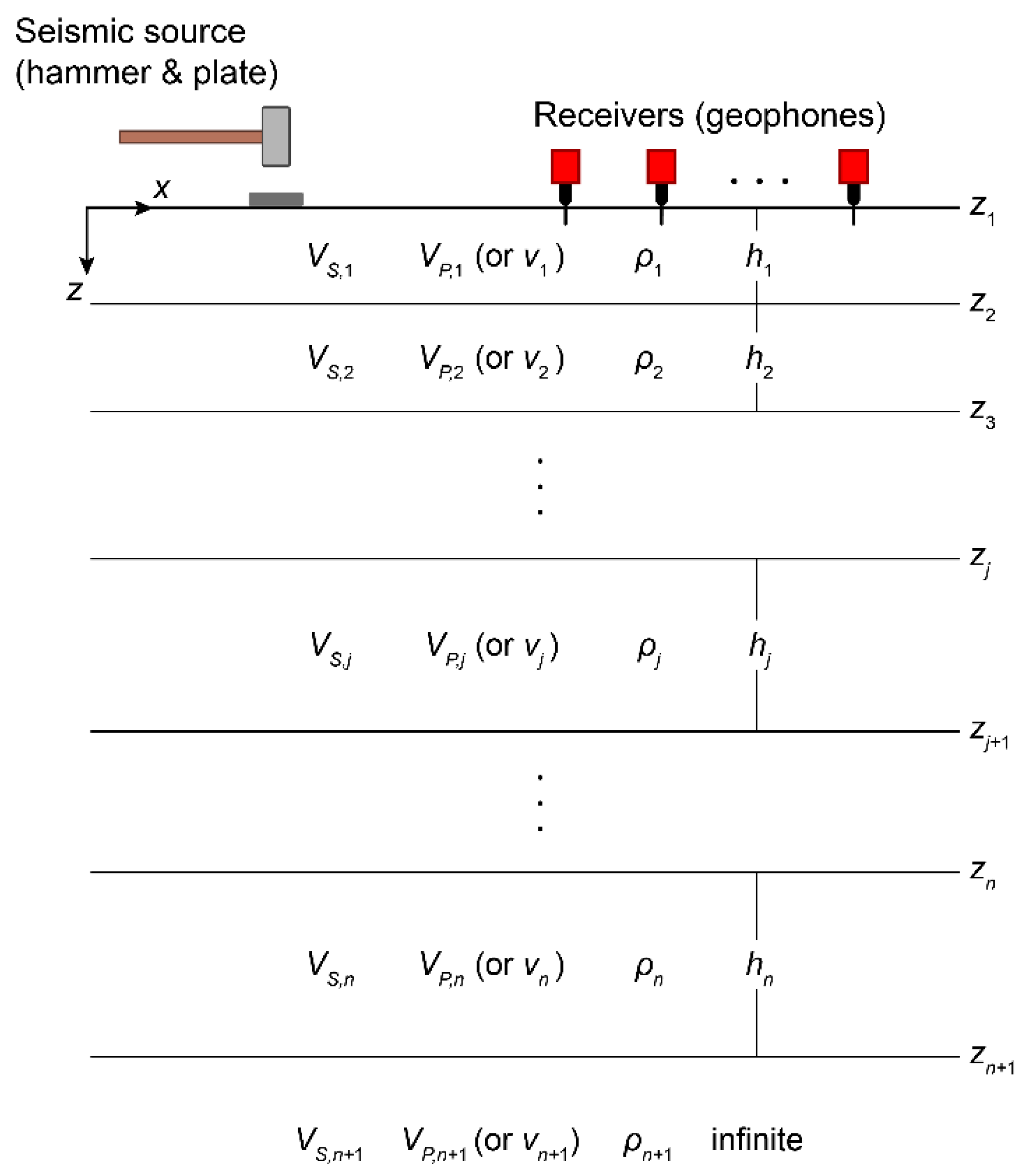
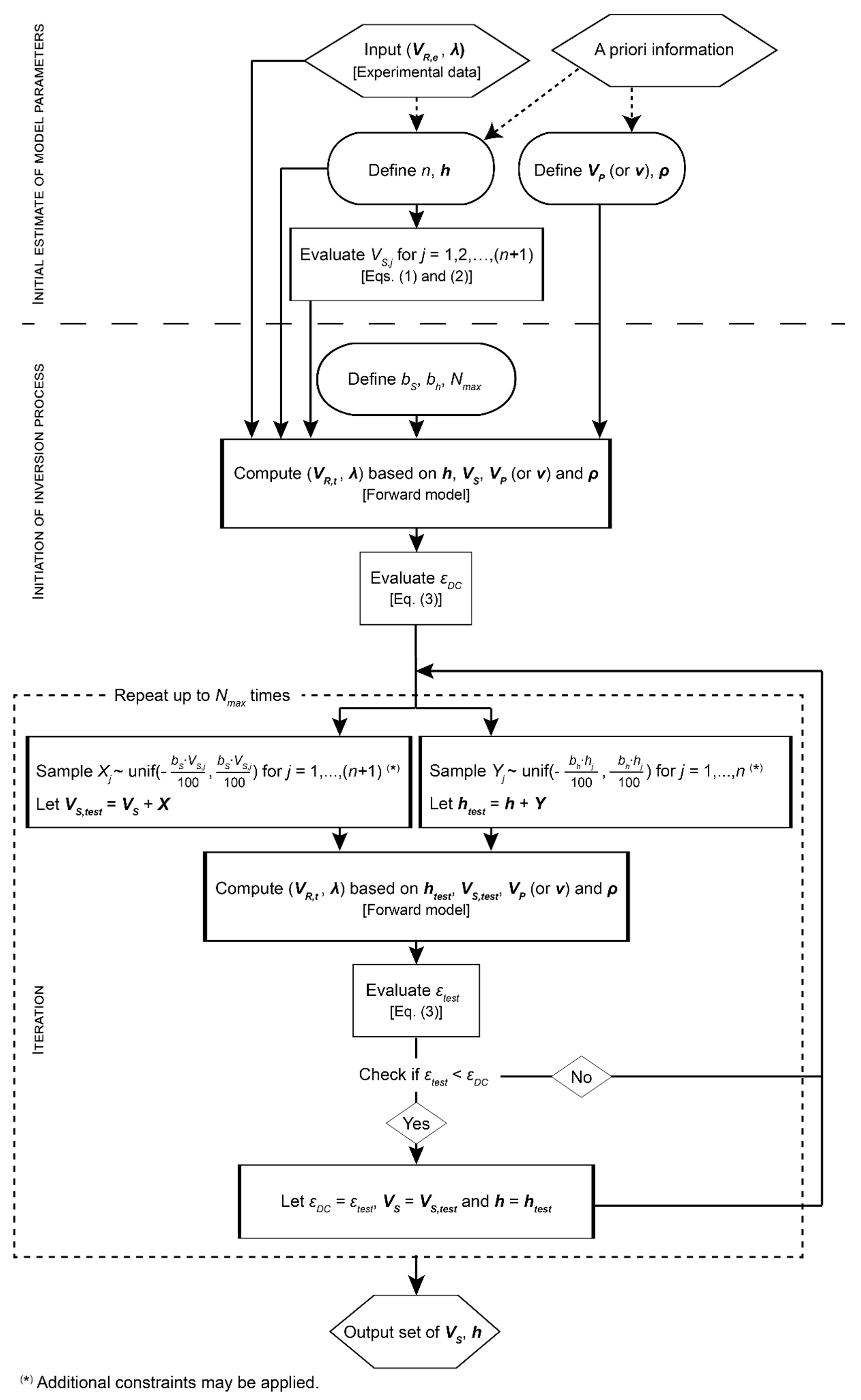
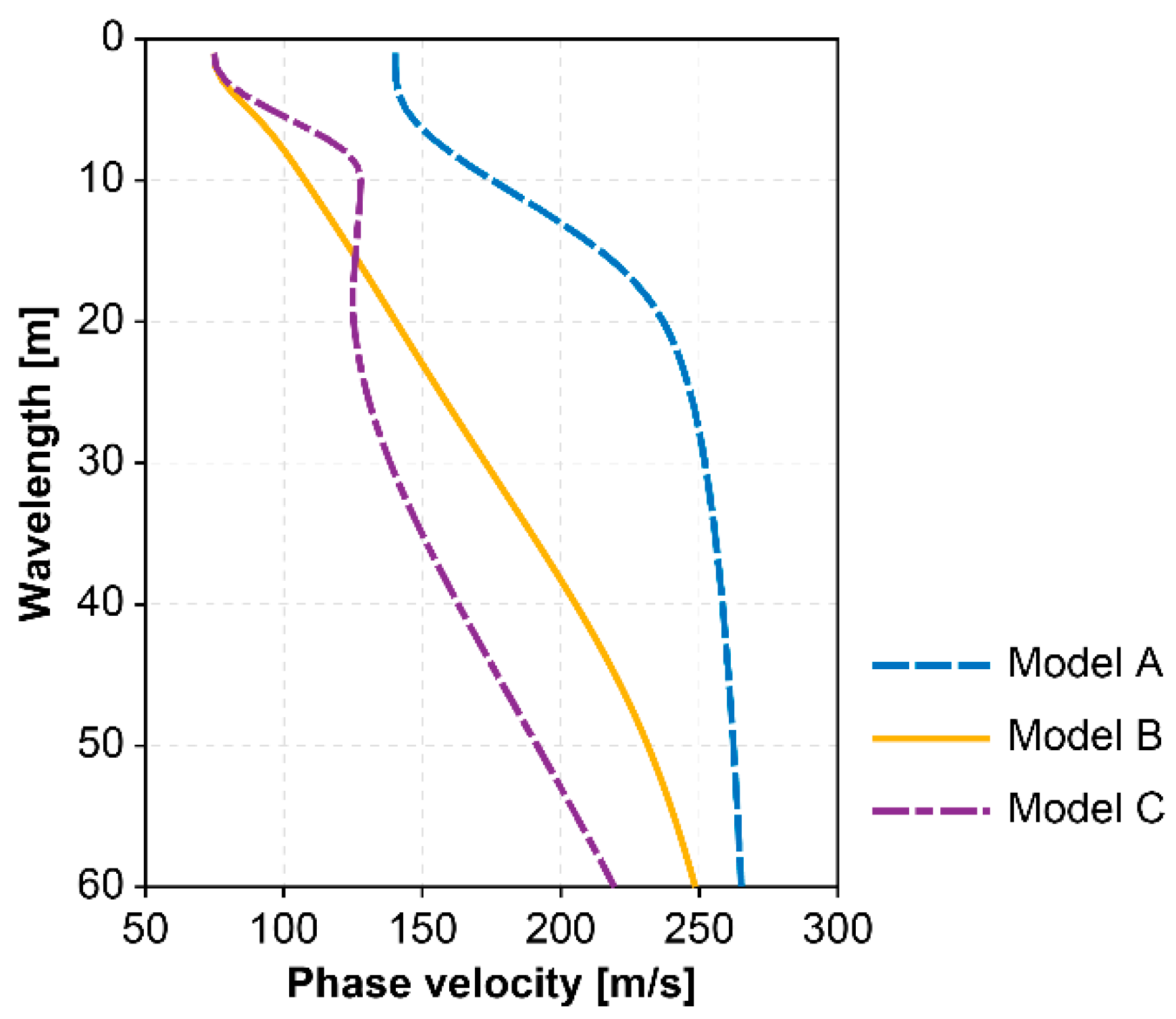
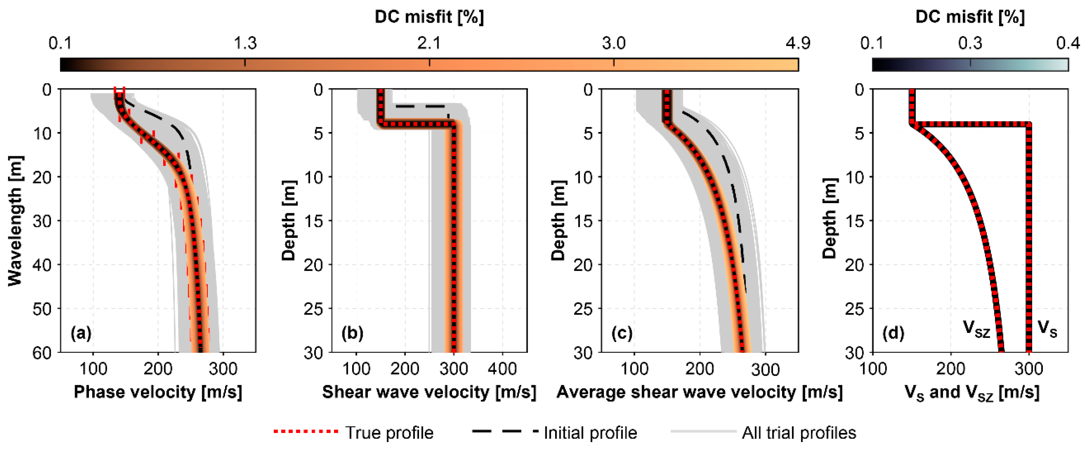
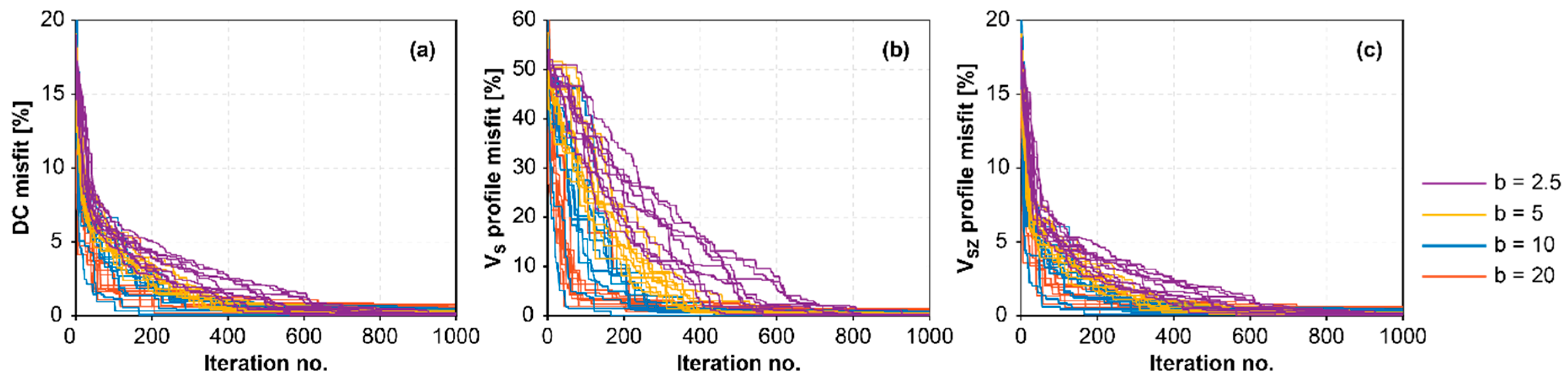
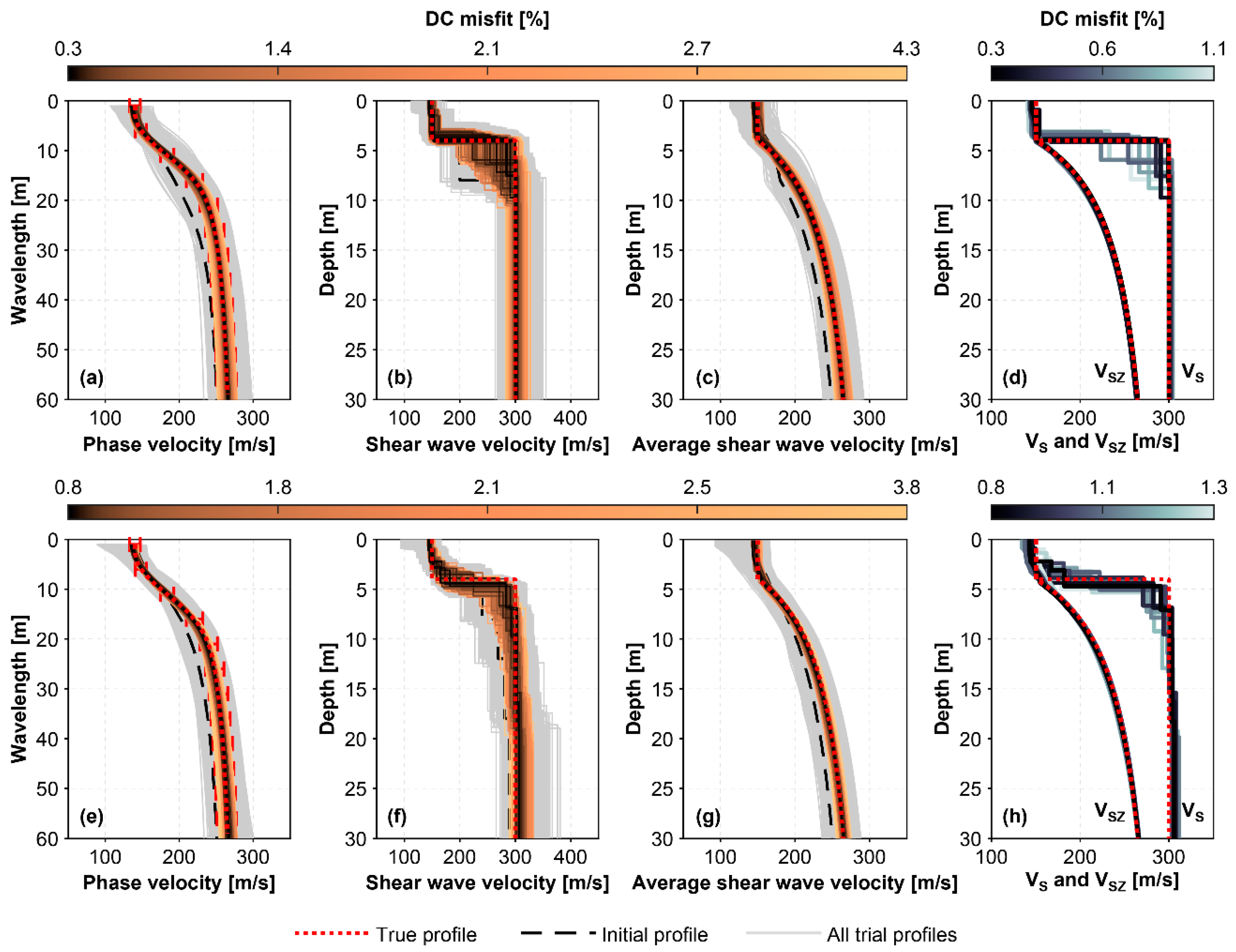
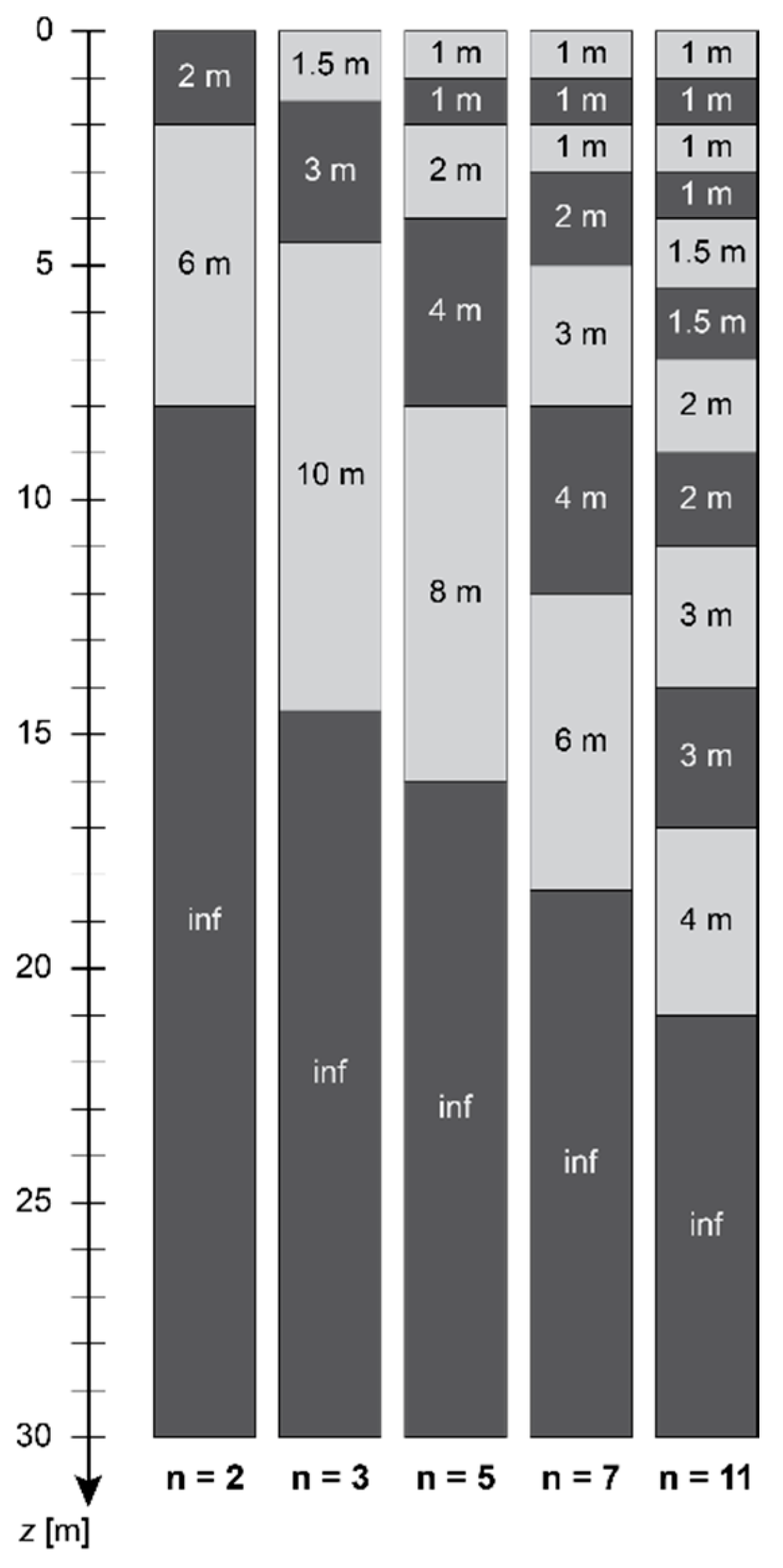
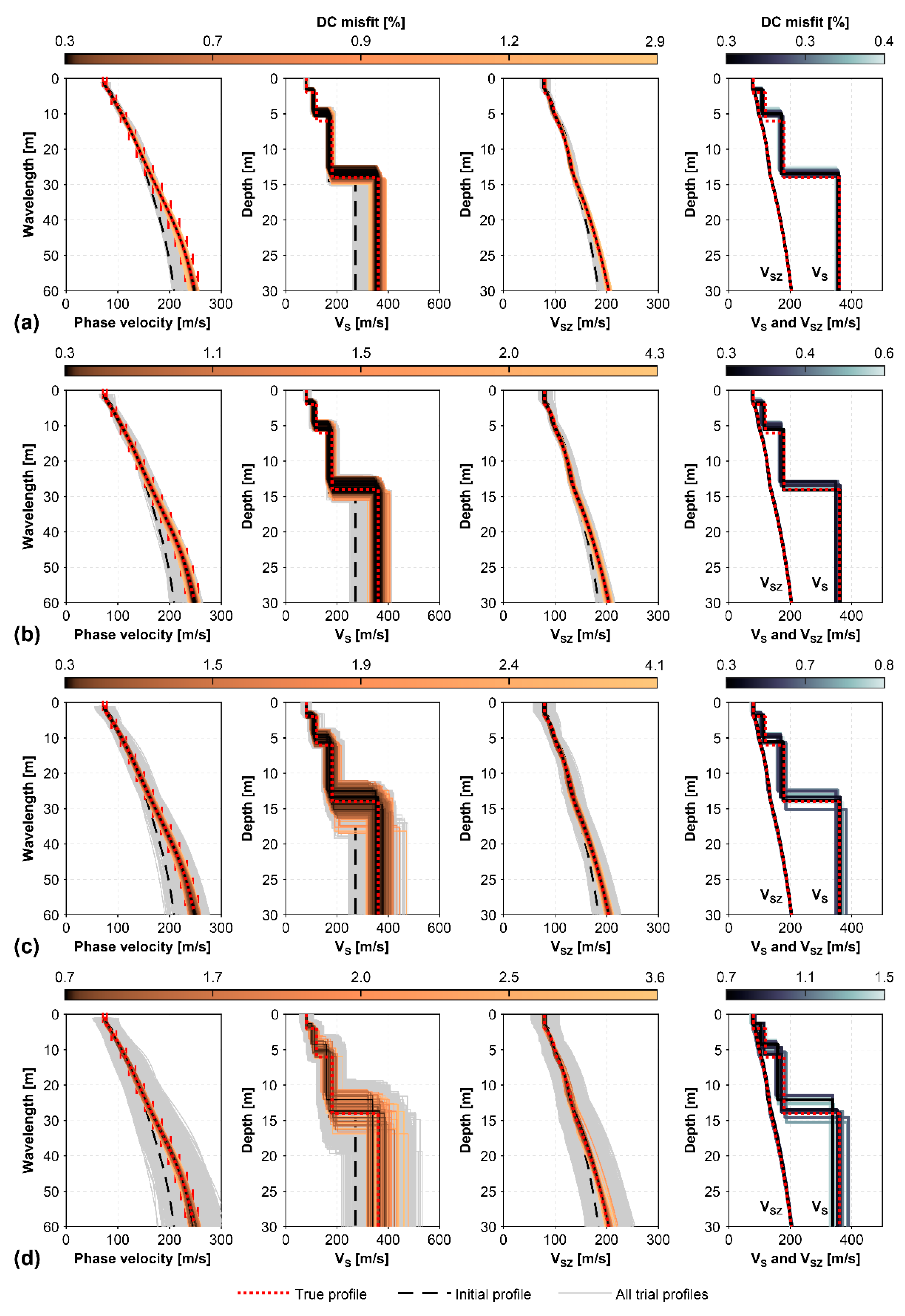
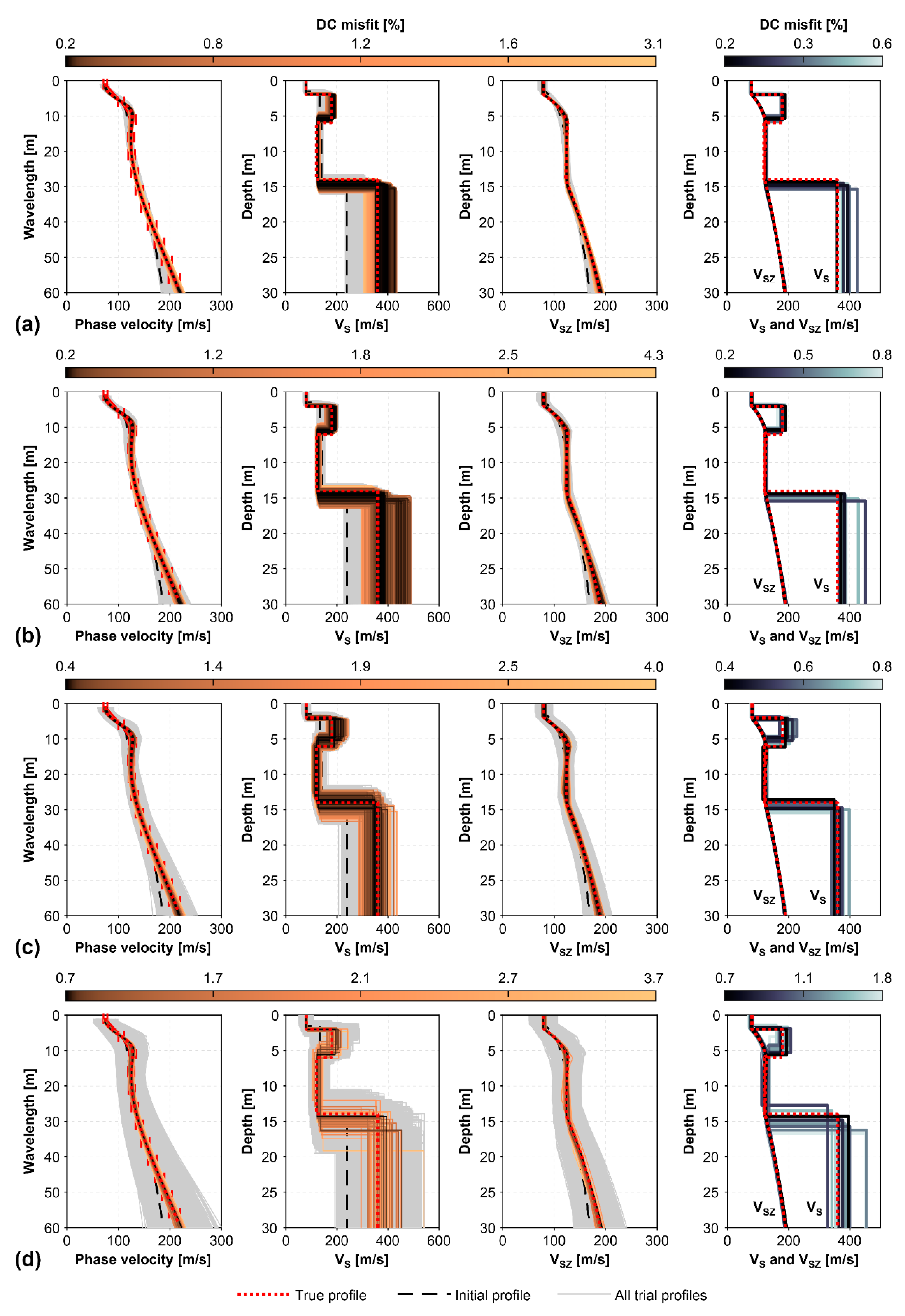
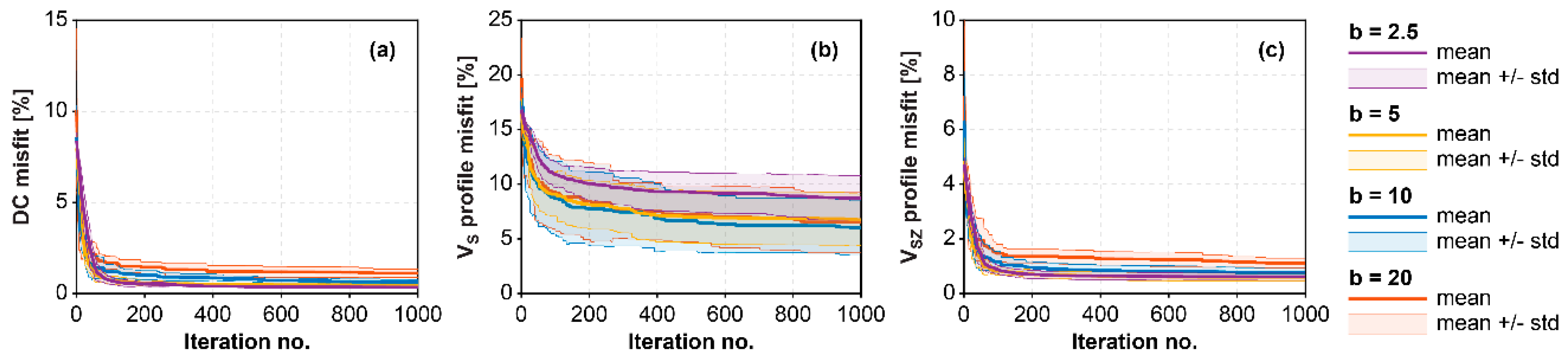
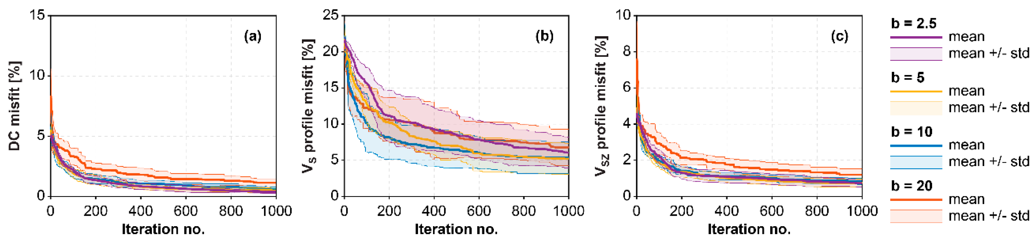
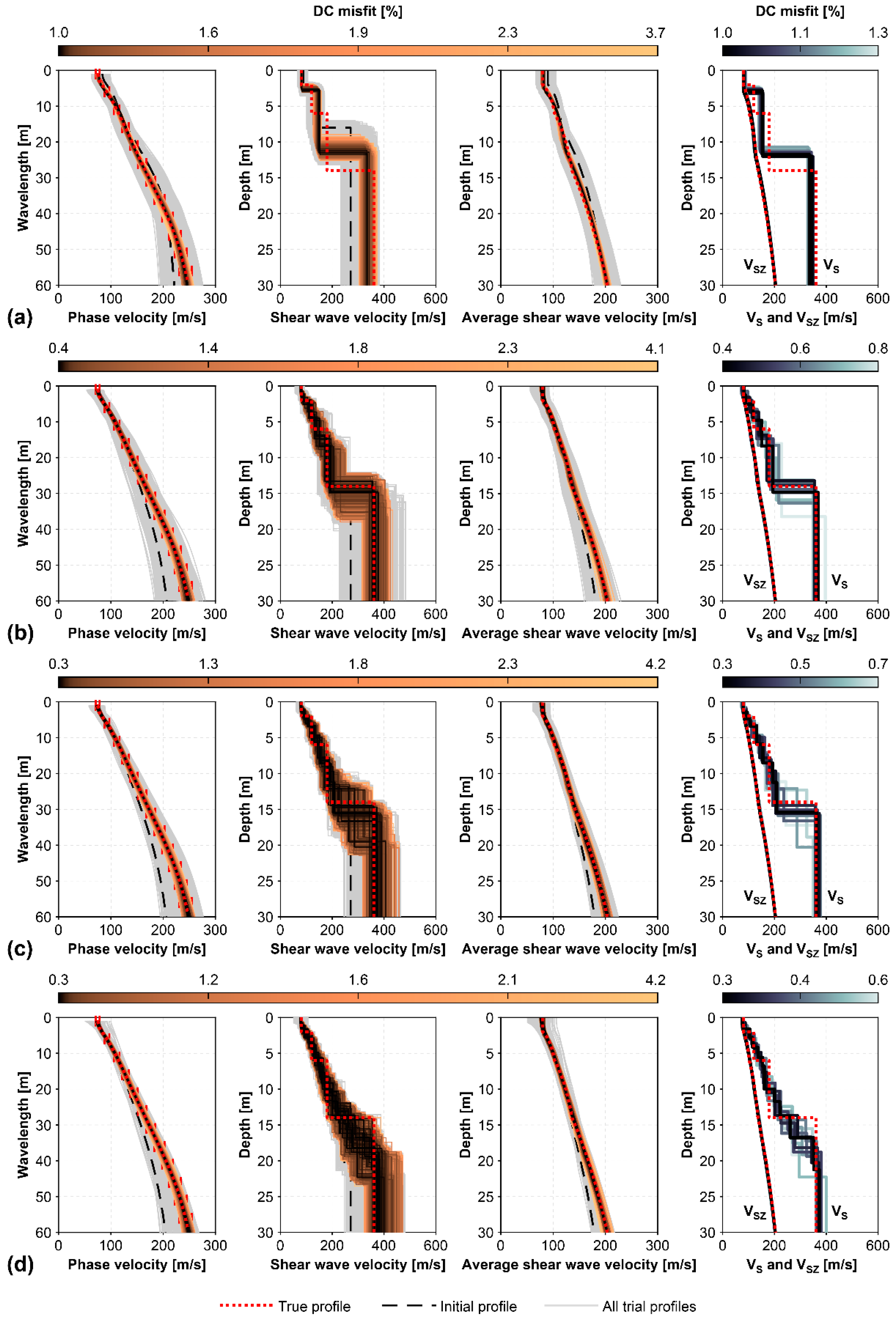
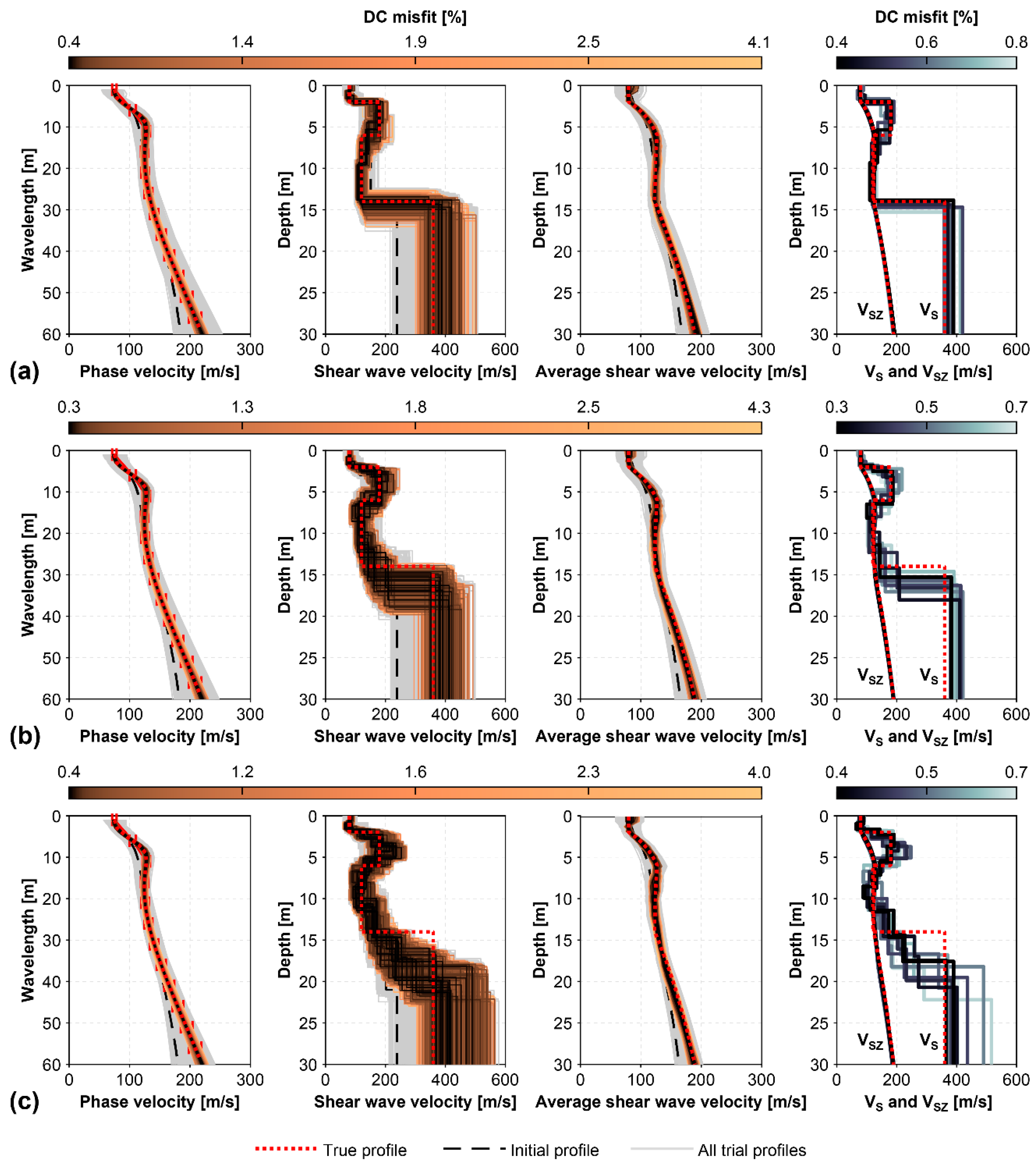
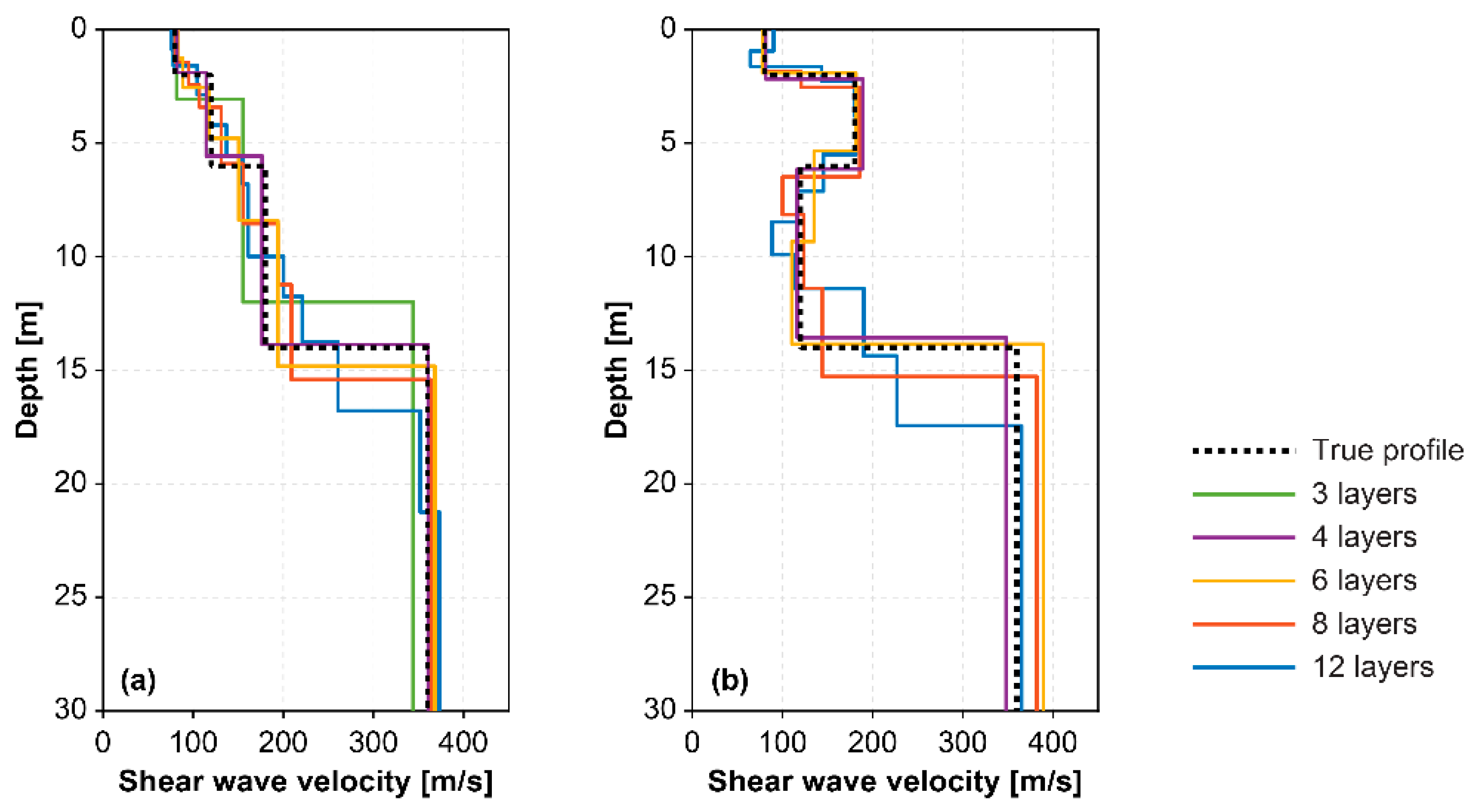
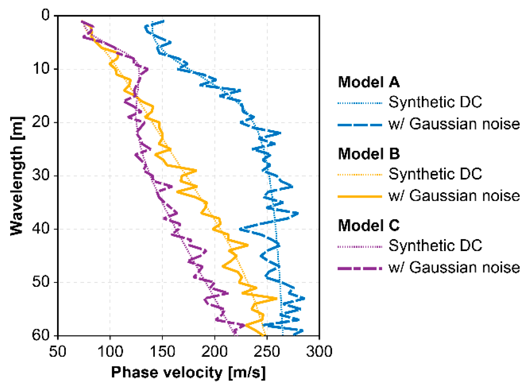
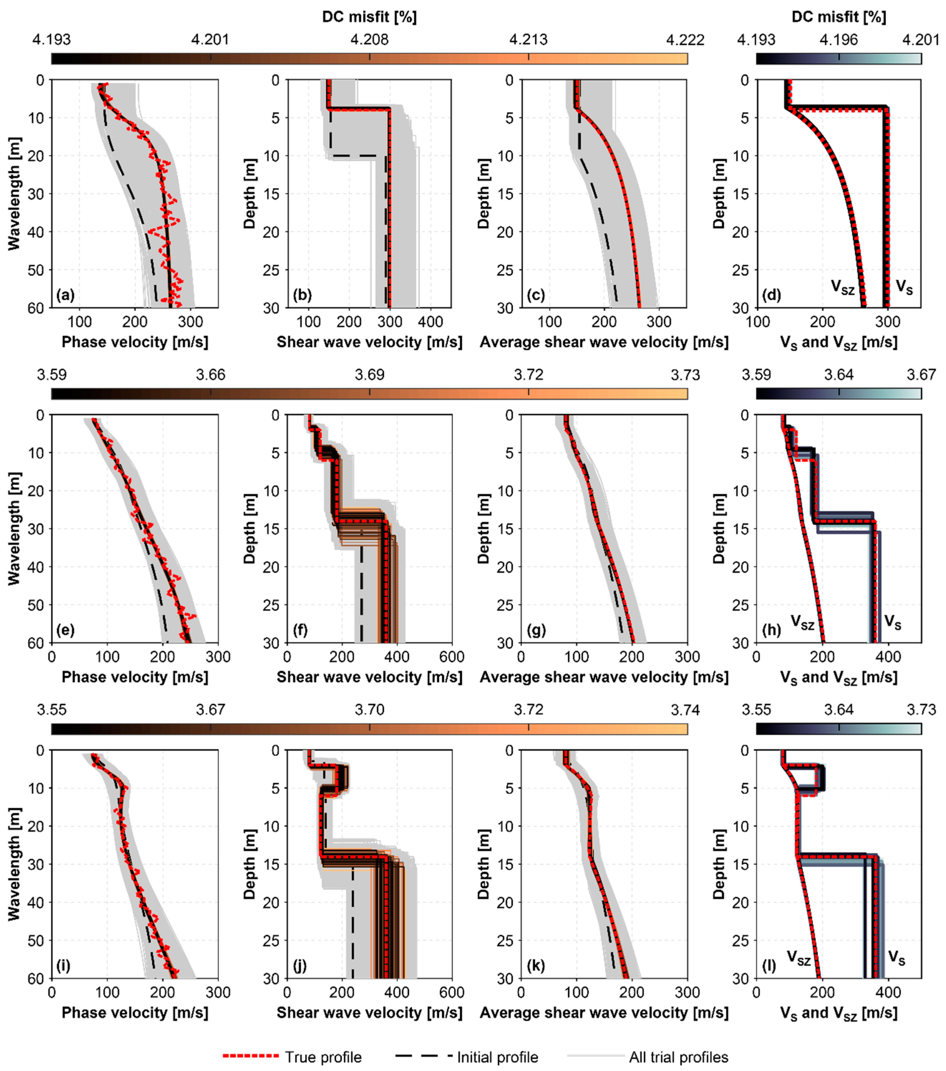
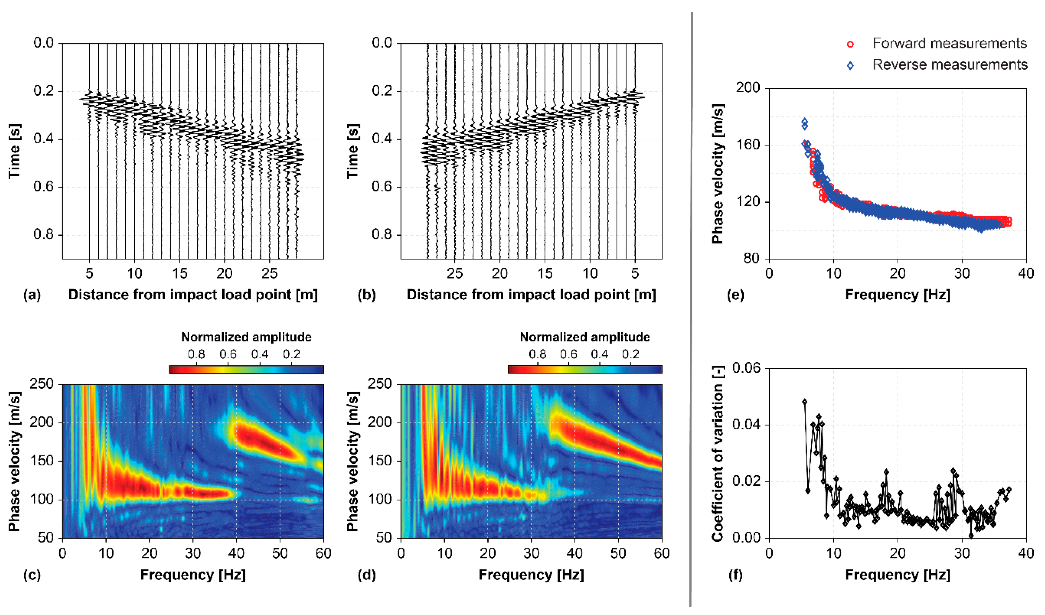
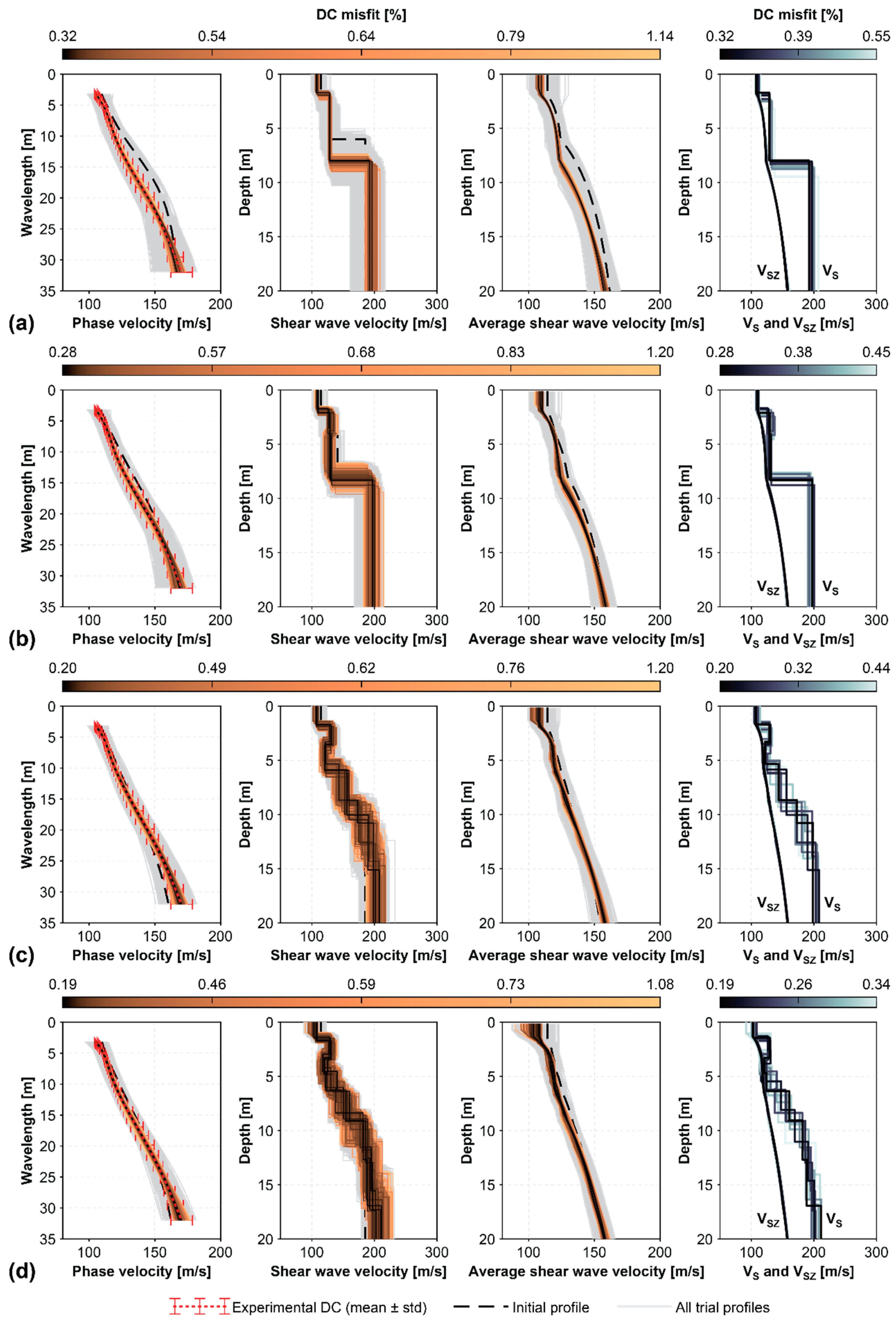
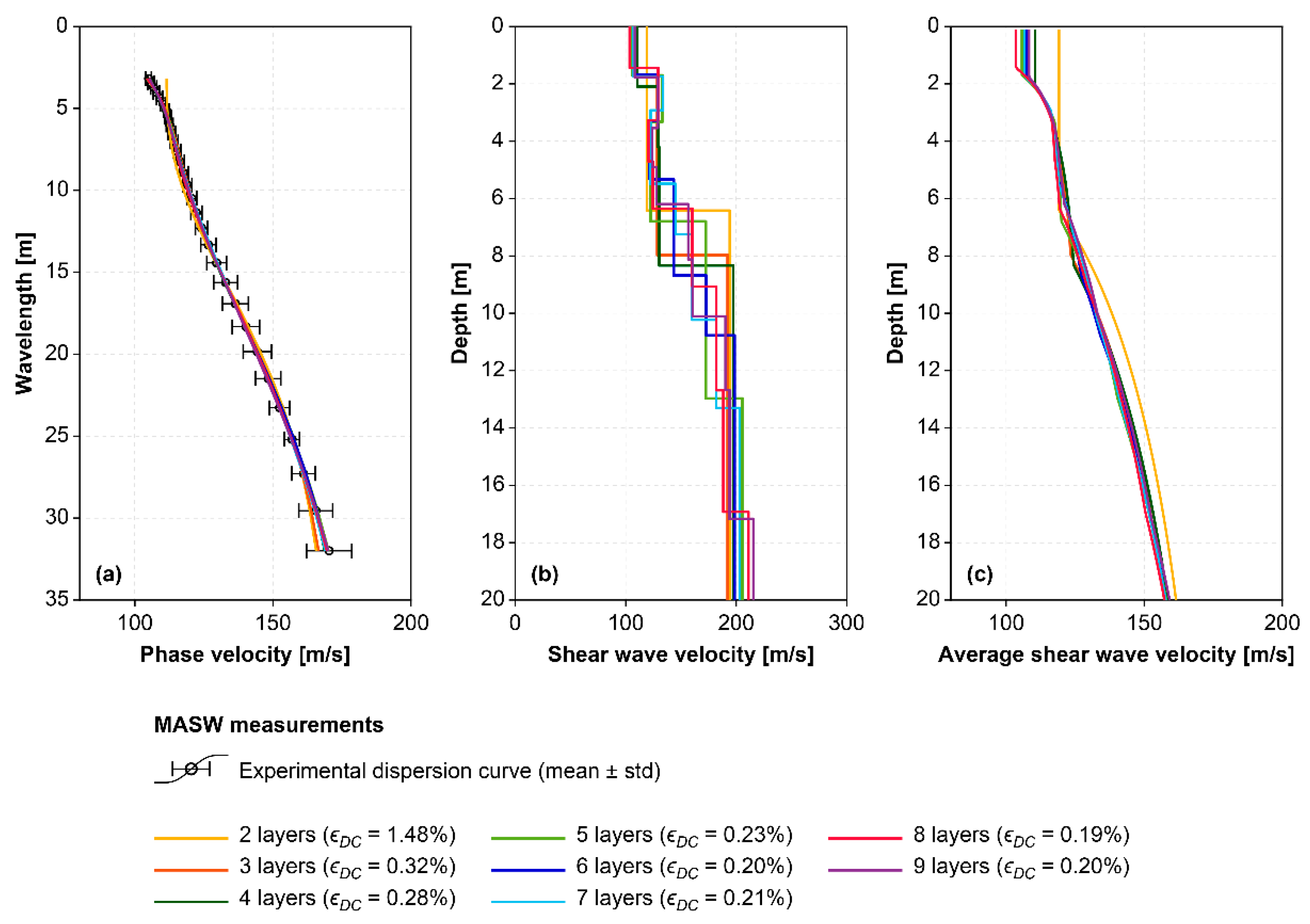
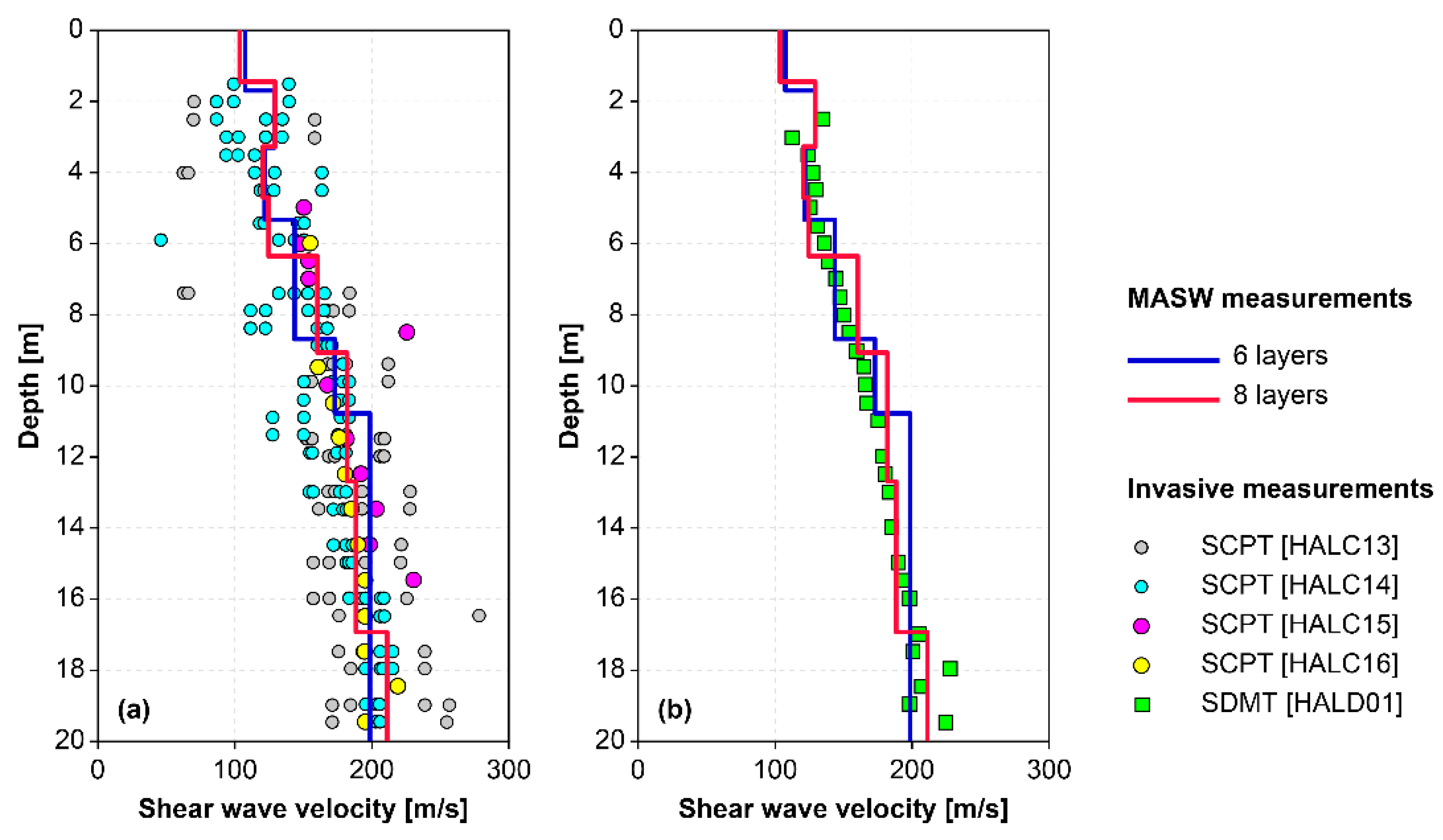
Table 1.
Model A, two-layer model characterized by an increase in shear wave velocity with depth.
| Layer Number | Shear Wave Velocity | Poisson’s Ratio | Density | Layer Thickness |
|---|---|---|---|---|
| [m/s] | [–] | [kg/m3] | [m] | |
| 1 | 150 | 0.35 | 1800 | 4 |
| (Half-space) | 300 | 0.35 | 1800 | - |
Table 2.
Models B and C, four-layer models characterized by a gradual increase in shear wave velocity with depth [model B] and a stiffer layer between two softer layers [model C].
Table 2.
Models B and C, four-layer models characterized by a gradual increase in shear wave velocity with depth [model B] and a stiffer layer between two softer layers [model C].
| Layer Number | Shear Wave Velocity | Poisson’s Ratio | Density | Layer Thickness | |
|---|---|---|---|---|---|
| [m/s] | [–] | [kg/m3] | [m] | ||
| Model B | Model C | ||||
| 1 | 80 | 80 | 0.35 | 1800 | 2 |
| 2 | 120 | 180 | 0.35 | 1800 | 4 |
| 3 | 180 | 120 | 0.35 | 1800 | 8 |
| (Half-space) | 360 | 360 | 0.35 | 1800 | - |
© 2020 by the authors. Licensee MDPI, Basel, Switzerland. This article is an open access article distributed under the terms and conditions of the Creative Commons Attribution (CC BY) license (http://creativecommons.org/licenses/by/4.0/).
Share and Cite
MDPI and ACS Style
Olafsdottir, E.A.; Erlingsson, S.; Bessason, B. Open-Source MASW Inversion Tool Aimed at Shear Wave Velocity Profiling for Soil Site Explorations. Geosciences 2020, 10, 322. https://doi.org/10.3390/geosciences10080322
AMA Style
Olafsdottir EA, Erlingsson S, Bessason B. Open-Source MASW Inversion Tool Aimed at Shear Wave Velocity Profiling for Soil Site Explorations. Geosciences. 2020; 10(8):322. https://doi.org/10.3390/geosciences10080322
Chicago/Turabian StyleOlafsdottir, Elin Asta, Sigurdur Erlingsson, and Bjarni Bessason. 2020. "Open-Source MASW Inversion Tool Aimed at Shear Wave Velocity Profiling for Soil Site Explorations" Geosciences 10, no. 8: 322. https://doi.org/10.3390/geosciences10080322
Note that from the first issue of 2016, this journal uses article numbers instead of page numbers. See further details here.