Linking Soil Hydrology and Creep: A Northern Andes Case
by
 ,
,
Aleen Pertuz-Paz
1,*, 
Gaspar Monsalve
1,
Juan Carlos Loaiza-Úsuga
1,
José Humberto Caballero-Acosta
1,
Laura Inés Agudelo-Vélez
2 and
Roy C. Sidle
3 1
Departamento de Geociencias y Medio Ambiente, Facultad de Minas, Universidad Nacional de Colombia, Medellín 050034, Colombia
2
Departamento de Ingeniería Civil, Facultad de Minas, Universidad Nacional de Colombia, Medellín 050034, Colombia
3
Mountain Societies Research Institute, University of Central Asia, Khorog 736000, Tajikistan
*
Author to whom correspondence should be addressed.
Geosciences 2020, 10(11), 472; https://doi.org/10.3390/geosciences10110472
Submission received: 13 October 2020
/
Revised: 8 November 2020
/
Accepted: 16 November 2020
/
Published: 21 November 2020
(This article belongs to the Special Issue Landslides and Granular Flows on Earth)
Abstract
:Soil creep is common along the hillslopes of the tropical Andes of Colombia, where very heterogeneous soils develop on old debris flow deposits and are subjected to abundant rainfall with a bimodal annual regime. In particular, the western hillside of the city of Medellín, Colombia, is comprised of a series of debris and earth flow deposits in which landslides and soil creep are common. To explore linkages between soil creep and hydrology, we selected an experimental site in the western hillslope of the Medellín valley to assess the behavior of water within the soil mass, its relationship with rainfall, and its connection with soil displacement. In experimental plots, we systematically measured runoff, percolation, water table levels, and volumetric water content, for a period of almost 2 years; we also conducted several alti-planimetric positioning surveys to estimate relative displacements of the soil surface. Moisture content of the soil remained above field capacity for most of the year (~68% of the time) and active and quasi-permanent lateral subsurface flow occurred within the upper 80 cm of the profile. The shallow flow likely facilitates the downslope movement. Additionally, our results suggest that displacement magnitudes are largest during the wet season of September–October–November, when a highly humid soil experiences changes in water content, so it is during this time that the effects of expansion / contraction of the soil particles (associated to wetting / drying cycles) contribute the most to the movement. This observational study represents a contribution to the understanding of soil creep in tropical hillslopes, where it responds to the wetting / drying cycles, with the particularities of a rainy weather (>1500 mm/year), warm temperatures (~22 °C on average), and a bimodal precipitation seasonality.
1. Introduction
The Tropical Andes of northern South America are highly susceptible to mass movements given the climate, topography, and susceptibility to soil erosion. The city of Medellín (Colombia) is located in the Aburrá Valley, with an average annual precipitation of about 1800 mm, slope gradients between 0° and 40°, alluvial deposits, and frequent debris flows along the flanks and at the base of the valley [1]. Currently the city is undergoing an accelerated transformation in terms of land occupation due to the economic and social changes that have led to the migration of people from the countryside and small urban centers into the main urban area. In the Aburrá Valley, irregular urban sprawl is concentrated on the high slopes; by 2010 there were 284,000 people at risk of landslide, and by 2030, there will be more than 344,000 [2].
Mass movements within the metropolitan region of Medellín and the Aburrá Valley exhibit a bimodal annual distribution, similar to that of the average monthly rainfall [3]. The two maxima for landslides occur in May and October, and both rainfall and mass movements increase during the latter rainy season. Along the western hillslope of Medellín the soils are mainly derived from debris flow deposits, whose granulometry covers all ranges, from gravels to clays [4], thus generating different structures, which strongly influence their physical properties and mechanical and hydrological behavior [5]. Soil creep is a common form of slope instability, which is defined as a slow motion modified and accelerated by small changes within the soil mass, often difficult to observe and demonstrate due to the lack of typical geomorphic features in the landscape [6]. However, in cases where soil creep is widespread and progressive, hillslopes often have hummocky topography and various vegetative indicators are evident, such as curved trees [7].
Mass movements are linked to complex hydrological systems, and as such, a simple relationship between rainfall and displacement is seldom evident [8]. Still, rainfall, infiltration, and the resulting variation in pore pressure can be considered the main triggers of the movement [8,9]. Therefore, an approximation to this relationship would help determine to what extent hydrology controls and affects erosive and deformational processes.
Uncertainties surrounding the triggering effects of rainfall on mass movements include the parameters for unsaturated flow in soils, such as diffusivity, soil moisture curves, the depth distribution of the soil profile, and the initial content of water, which are generally unknown, but are sensitive parameters in soil hydrology models [10]. Thus, it is imperative to know the soil moisture conditions before starting the precipitation event and to define their role in the instability [11].
Here, we relate the hydrological dynamics of the soil to the stability of a visibly affected hillside from a geological, geomorphological, and pedological perspective. Subsequently, we focus on characterizing hydroclimatological variables such as precipitation, runoff, percolation, piezometric levels, and soil moisture, to explore their relationship with the creep phenomenon. It should be noted that soil moisture, in hydrological dynamics, is the key variable that synthesizes the interactions of climate, soil, and vegetation within the water balance [12].
Within the framework of this research, it is noted that mass movements such as landslides, debris flows, and subsidence, among mass movements, can be triggered by soil creep and its response is accelerated by rainfall [13,14,15,16]. For this reason, the analysis of the different processes in the climate-soil system depends on the temporal and spatial scales addressed. Thus, the hydrological response of the soil was analyzed weekly and biweekly and at the plot scale (a few meters); a basic level of analysis of the climate–soil–vegetation system [12].
Despite the clear hydrology–deformation relationship for the soil, there is a lack of spatially explicit data and calibrated models to illustrate how it influences slow-motion landslides [9]. Soil creep research is highly concentrated in regions of mid and high latitudes, and studies in tropical regions, particularly in South America, are rare [6]. A recent study reported some initial observations on an experimental site in the western hillslope of Medellín, including a general geophysical characterization of the subsurface and some first order hydrological measurements, suggesting that constant soil saturation and relatively shallow subsurface flow play active roles in the soil creep [17]. As a follow up, this study describes a more elaborate hydrological data set at the same site and aims to characterize the motion itself and its relationship with the soil hydrology using qualitative observations and quantitative relative positioning measurements. These observations will allow us to infer some aspects of how the well-known soil creep mechanisms [18] are linked to the hydrological characteristics of this mountainous tropical area and to the associated soil response.
2. Field Site Description
2.1. Geology and Geomorphology
The Aburrá Valley is the result of a complex tectonic evolution, and its landscape has been significantly modified by weathering. The alluvial and slope deposits occupy a considerable extension within the valley and are mainly associated with the Medellín River and its tributaries [4]. The locality of El Yolombo, on the western slope of Medellín, at elevations between 2100 and 2600 m.a.s.l., was chosen for this investigation (Figure 1). In this area, stability problems and numerous mass movements are evident, mostly landslides, soil creep and earthflows, that occur on slopes where older debris flow deposits appear [17]. The main depositional feature in El Yolombo has a wide range of grain sizes, from clay to heterometric blocks of gabbro and amphibolite; the soil matrix to rock ratio is between 40% and 60%, with angular pebbles prevailing among the blocks [17].
Slope gradients mainly range between 15° and 30°, with some flat sectors that favor water accumulation; the shape of the hillslope is generally straight to concave. The landscape in the area is characterized by a hummocky topography, defined as a set of mounds separated by irregular depressions that lack linear or lobed shapes, and do not align on ridges [19] (Figure 2). These mounds and depressions, in addition to being the product of denudation, are also generated from the accumulation of material displaced by creep (Figure 2). This slope heterogeneity can be highly controlled by the movement and distribution of water and suggests that the soil moisture regime is highly variable [20,21].
The experimental site (Figure 1) is located in an area of about 3 ha with slopes between 5° to 30°, steeper in its northern part; in the southern portion, the landscape has been smoothed by denudation and anthropic activity (mainly minor cattle grazing), with greater water accumulation. Geologically, the site is composed of slope deposits, landslides, and torrential alluvium associated with a creek located on the east side of the study area. On the surface, accumulation of angular to subangular blocks up to 1 m in diameter are present, as well as terracettes, furrows, subsidence, some slide scars, and material detached in the northern part (Figure 2a–d). Both rapid mass movements (landslides, rock falls) and slow ones (creep) are evident, and there are possibly deeper processes, as previous geophysical experiments report a major discontinuity between 4 and 6 m [17]. This discontinuity is probably related to the contact between two debris flows with significant differences in age and compaction; such surfaces can facilitate the downhill sliding and suggests that hillslope processes are occurring on the surface as well as at depth.
2.2. Pedostratigraphy
The soils in the study area were characterized as inceptisols, and classified as clay–skeletal, kaolinitic, subactive, isothermic Typic Dystrudepts [22], corresponding to the Tequendamita association [23]. They developed from metamorphic and intrusive rocks, such as amphibolite, gabbro, gneiss, schist, and phyllite, and may contain intermingled volcanic ash. The soil profile has a low pedogenetic development, consisting of a sequence of colluvial deposits. The shallow organic mineral layer overlies a sequence of heterometric deposits with a fine matrix (silty clay to clay), whose percentage decreases with depth.
The uppermost horizon (Ap) can be as thick as 40 cm, has a loamy clay texture and medium subangular block structure, rich in organic matter and fragments of roots and tissues. The underlying horizons correspond to 2Bw1 (~40–60 cm thick), 2Bw2 (~70–80 cm thick), on top of 3BC and 3C horizons around 1 m thick. Figure 2e,f shows the soil profiles in trenches at the plot locations. The boundaries between all horizons are very abrupt and clear fine materials, with iron oxyhydroxides, iron, and manganese nodules are very evident in the upper 1.2 m of soil. Fe depletions, Fe-Mn impregnated hypocoatings and nodules are related to redox environments [24]. Medium to fine textures predominate (silty clays to clays), but gravels and stones are common, as well as layers of iron oxides. Rock fragments within the soil mass have diameters between 10 and 40 cm. Colors vary from olive brown to olive gray. The diameter and percentage of rock blocks, fine textures, and grayish colors (gleyed soil) increase with depth.
Soils in the area show evidence of erosion due to diffuse runoff, furrows, cattle tracks, and localized mass movements. They are moderately acidic, have low fertility, high contents of iron and aluminum, high to low cation exchange capacity, medium to low total base at the surface and shallow depths, and low base saturation; organic carbon decreases from low at the surface to very low at depth. These soils are typical of those in the premontane wet forest life zone bh-P (wet coffee lands) [25]. The primary vegetation has been removed giving rise to forest plantations mixed with grass and stubble, and the site is currently used for livestock and marginal agriculture production.
2.3. Soil Creep
Slow-moving landslides are found in various climatic and geological environments, and when examined in detail, it is difficult to infer direct relationships between precipitation, slope gradient, and rate of movement. However, these slow mass movements often exhibit a seasonal pattern of acceleration and deceleration [7,9]. Soil creep is determined and modified by climate (temperature and soil moisture conditions), biota, topography, rock weathering processes, and soil production rates [6,26]. With the first objective of characterizing the movement type, a qualitative description of the phenomenon that affects the stability of the slope was conducted.
Continuous creeping is a phenomenon that occurs below the surface and the shallow zone of seasonal variations, and depends on the viscosity and rheological properties of the soil. On the other hand, seasonal creeping occurs superficially and depends on fluctuations in soil moisture (wet and dry periods), rock, regolith and soil changes due to weathering, and short-term increases and/or decreases in loading on the soil surface. Thus, we can assume that seasonal soil creep occurs on top of the continuous creep zone [6,27,28]. In this research, we focus on seasonal soil creep, which is highly controlled by the slope angle, curvature of the topography, soil depth where hydroclimate exerts a major control (to about ~0.80 m depth), soil texture and density, and fluctuations of moisture within the soil. We also assume that creep can precede or follow other mass movements such as landslides and/or earthflows [6,13,14].
Along the slope, recent evidence of creep was found, including cracks in roads, damaged containment structures, bent trees due to deformation of roots by the downhill movement of the soil, and damage to houses (Figure 3a–d). At the hillslope scale, evidence of soil displacement was found in the terracettes where scars or cracks were observed, and in the mounds that are the product of accumulation of mobilized material (Figure 2a–d). The latter, in most cases, were not aligned and smoothed by denudation, and the depressions are irregular, consistent with the characterization of the hummocky landscape [19]. At the pedon level, rock blocks of centimetric dimensions and subangular shapes (Figure 3e,f) were found integrated within the organic matter horizons; thus, we infer that this mixture could have occurred as a result of the movement. It is presumed that these rock blocks, which are also observed on the surface, are exposed by the weathering of the slope deposit and/or come from a pre-existing scarp upslope.
Although a variety of mechanisms could be at play to generate soil creep, expansion and contraction processes within the soil mass, associated to changes in soil moisture, have been addressed as one of the main causes [18,29,30]. Stresses associated to soil expansion take place in a direction perpendicular to the surface, and those associated to contraction occur in a nearly vertical direction [18]. This may result in a zigzag movement of soil particles, roughly following the slope direction, without scars or a single surface of rupture [29]. Given the hydrological regime at the study site, with the soil wetting and drying cycles operating in an annually bimodal fashion, the associated expansion and contraction of the soil particles should also be linked to the annual hydrological cycle.
3. Data and Methods
3.1. Hydrological Instrumentation
A total of 2 experimental runoff plots were installed at the study site (Figure 1d) with areas of 4 m2 (plot 1) and 1.6 m2 (plot 2), according to a previously established methodology [5]. In addition to runoff, lysimeters were installed to estimate percolation. The site was monitored from March 2018 through December 2019. The measurement campaigns were conducted weekly; however, given the logistical limitations at the beginning of the monitoring process, visits were sometimes biweekly and in some cases it was not possible to regularly take samples. Therefore, the data were limited to 2 time windows: March to May 2018 and August 2018 to December 2019.
For percolation estimates, we used zero tension lysimeters [32], which were installed according to the edaphological and geomorphological characteristics of the slope. These consisted of rectangular boxes of 0.2 × 0.3 m, designed to collect the flow that infiltrates into the soil profile, both by direct percolation from the surface and by lateral subsurface flow. Finally, a total of 4 lysimeters (2 per plot) were installed at different depths, 2 within each runoff plot, according to the description of the soil profile. Table 1 shows the main characteristics of the runoff plots and the associated instrumentation, including the capacity of the tanks that collect runoff and percolation water. The capacity of the tanks limits the maximum values of runoff and percolation that can be measured, so the scale of the data might be saturated for some measurements during the rainy periods. During the course of monitoring, the deepest lysimeter in both plots collected the largest amount of weekly water. A total of 4 open-type piezometers [33] were installed along the studied slope (see Figure 1d for locations) to monitor shallow water tables in the soil. These were constructed from PVC pipes with a length of 1.50 m. Figure 4 shows photographs of one of the two runoff plots and one of the piezometers.
At the point scale, where Trench 3 (Plot 2) is located (Figure 1d, Figure 2f), soil moisture was measured from October 2018 to December 2019. In total, 4 ECH2O-EC5 sensors (Decagon Devices Inc., Pullman, WA, USA) were installed vertically at depths of 0.2, 0.4, 0.6, and 0.80 m, which correspond to the identified soil horizons and their textural differences: the shallowest sensor was at the base of the Ap horizon and the other 3 were located within the 2Bw1 horizon (Figure 2f). These sensors measure volumetric content of water in the soil (m3/m3) and the data were stored at 15-min intervals, using a EM-50 Data-logger (Decagon Devices Inc., Pullman, WA, USA), and compiled in a daily time series. To calibrate the 4 sensors, soil cores were collected in situ at depths of 0.2, 0.4, 0.6, and 0.80 m, the water content was measured, and gravimetric moisture content was estimated for each of them. This soil moisture was compared with the sensor readings and the calibration was performed through linear regression, with a determination coefficient of 0.67, and a measurement precision of ±7%. To contextualize the results obtained from monitoring soil moisture, and to relate them with its hydraulic properties, such as field capacity and permanent wilting point, we used ternary diagrams, which are a function of the percentage of sand, silt, and clay [34]. Likewise, to determine the degree of volumetric saturation of the soil, we used an approximation from the soil texture [35]. Table 2 shows the soil moisture conditions for the four sensors according to the Volumetric Water Content.
The discussion of the behavior of piezometric levels, runoff, percolation, and soil moisture was conducted based on the analysis of precipitation, which occurs in the study area throughout the entire year with maxima in March and October. This meteorological information was collected from 2 climate stations located 0.6 km and 3 km from the monitoring site. A study by Bedoya-Soto et al. [36] shows a very consistent behavior among rain gauges in the area in terms of the mean annual and diurnal cycles of rainfall, so we infer it is safe to use data from these 2 stations as a proxy to rainfall on the study site. They have 2 rain gauges each and rainfall is recorded every minute; the information is collected in the database of the Early Warning System of Medellín and Valle de Aburrá (SIATA). It should be noted that the precipitation series is compiled on a daily basis and due to the variable quality and availability of data, the 2 stations were processed.
In the results of this work, data are presented exactly as they were taken in the field, so as long as a measurement was successfully collected, it was reported and added to the time series. The basic statistics (mean, standard deviation, median, and 25 and 75 percentiles) of the collected data at plots and piezometers are shown in Tables S1 and S2 of Supplementary Materials.
3.2. Positioning Surveys
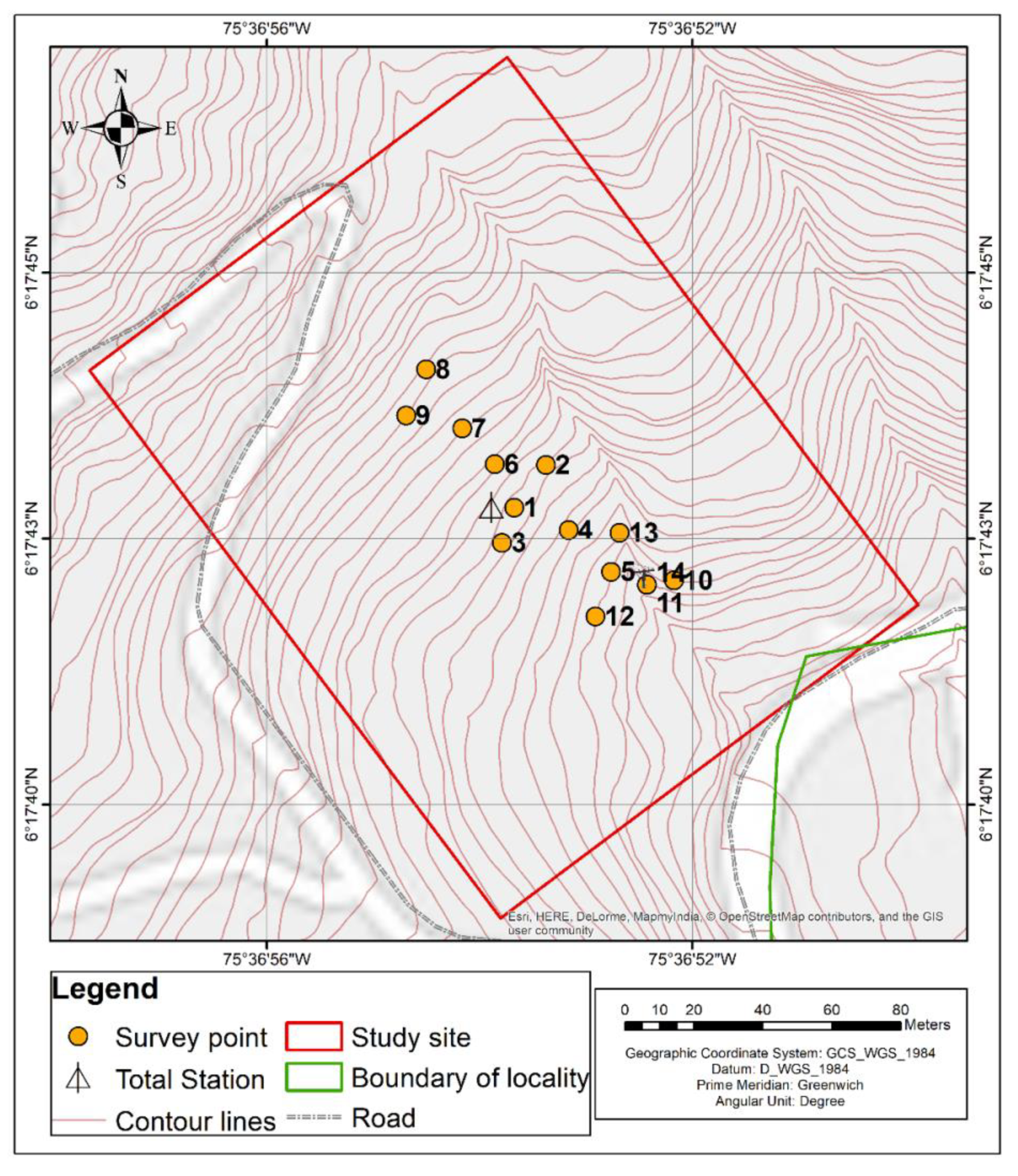
To better characterize the deformation of the terrain and the relative displacements, a systematic alti-planimetric survey was conducted. Our choice of measuring relative motion was due to the difficulty of finding a stable location on the hillslope. For the measurements of relative positions, we used a Topcon total station, during 6 campaigns between June and December 2019; these surveys were intended to be conducted monthly (26 to 35 days between field campaigns), but during August we were unable to go to the field (Table 3). A total of 13 cylindrical concrete benchmarks were installed as survey points (Figure 6); their length was 0.35 m. In each survey, we took North, East, and elevation (Z) coordinates with respect to a point within the study site (triangle in Figure 5), so the measurements correspond to relative position between 2 creeping points. To observe the evolution of relative soil displacement in different periods, the difference in survey position between 2 consecutive field campaigns was taken; such differences were calculated as the Pythagorean distance between 2 points. The estimated uncertainty in the relative position is associated to the nail diameter on the total station fixed survey point and on the benchmarks of the measuring points, which affect the location of the total station’s laser; this was estimated to be 10 mm. The basic statistics (mean, standard deviation, median, and 25 and 75 percentiles) of the collected positioning data are shown on Table S3 of Supplementary Materials.
4. Results
4.1. Hydrological Behavior: Water Table, Runoff and Percolation
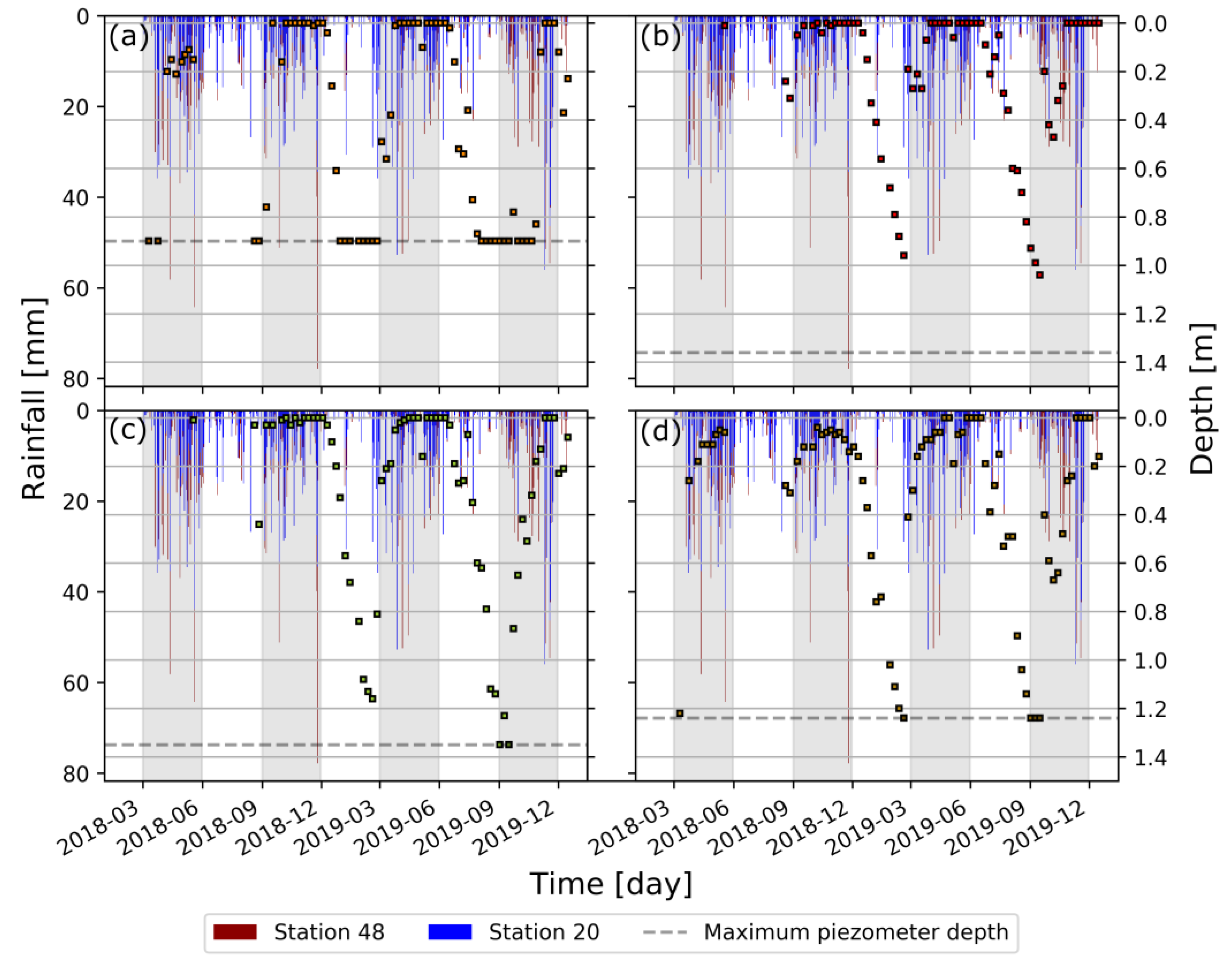
Water table fluctuations are closely related with precipitation (Figure 6). During wet periods, the water table oscillates mostly between 0 and 0.4 m below the surface. During dry periods the water level decreases gradually and may reach levels below the bottom of the piezometers (Figure 6b–d); when the rainy season starts, it can take several weeks to detect a response, which ultimately rises close to the ground surface. Notably, this response was slower during the last wet period of 2019 (Figure 6). The water table ascent is controlled by the volume and periodicity of the rainfall; it then remains at the surface until the end of the wet season and in some cases this behavior extends to the dry season for up to 3 weeks. Even though the piezometers are most likely recording a perched water table [17], it is clear that for most of the year, its level is above 1 m depth, and for nearly 70% of the time it is above 0.4 m. According to the most recent Aburrá River basin development planning and management study [37], and based on 25 years of data taken at a station within 3 km from our study site, the real evapotranspiration is quite homogeneous throughout the year: its value during the dry months of the year (June–July–August and December–January–February) does not surpass that of the wet months by more than 10%. This means that fluctuations in the water table are mainly linked to the variations in rainfall rather than increases in evapotranspiration during the dry periods.
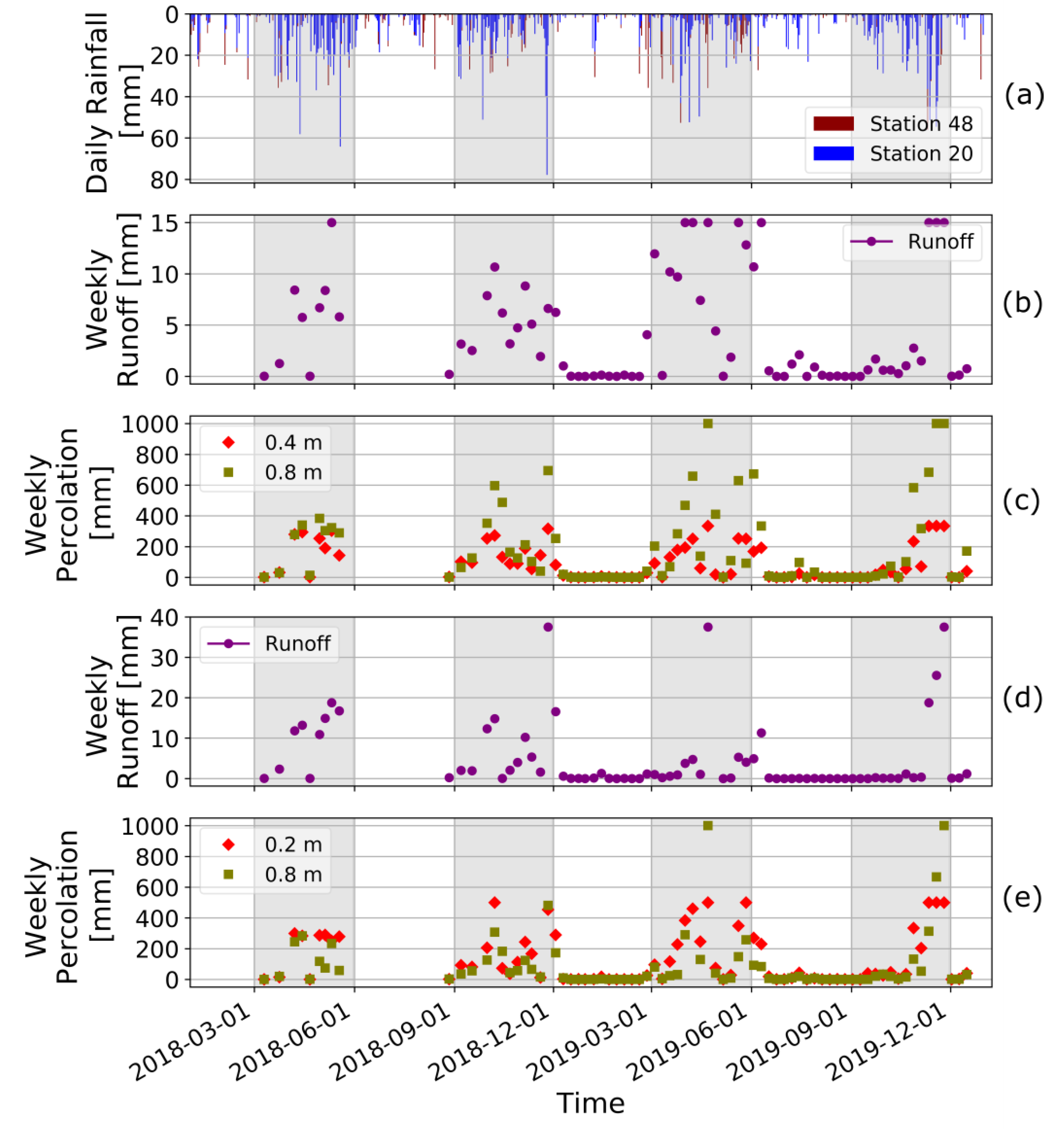
Figure 7 shows the behavior of runoff and percolation in the two experimental plots of our study site; the time series of both variables suggest a positive correlation with the rainfall. For the rainy periods, runoff reached a maximum of 37.5 mm/week (Figure 7b,d) shortly after rainfall events greater than 50 mm/day. Runoff values greater than 10 mm/week are in general associated with previous rainfall events greater than 20 mm/day; the lowest values of runoff (nearly 0 mm) are generally associated with dry periods and, in some cases, this behavior extends into the wet season. This is particularly noticeable for the last transition from dry to wet season in 2019 (Figure 7b). The mean runoff values for the wet seasons are about 5.3 mm/week.
For the shallowest lysimeters (0.4 and 0.2 m in plots 1 and 2, respectively), the highest values of percolation ranged from 333 to 500 mm/week (Figure 7c,e), associated with weekly rainfalls typically greater than 60 mm and daily precipitation values that in some cases exceeded 50 mm. Percolation values greater than 140 mm/week are normally associated with weekly precipitation values greater than 20 mm. In general, percolation at these shallow levels is nearly zero during the dry season, and then responds to continuous precipitation events of more than 5 mm/day. About 90% of the rainfall episodes record < 20 mm/day; in this case, the main factor that determines the volume of percolated water is the rainfall frequency rather than intensity (Figure 7a,c,d). Percolation values at 0.8 m below the surface are larger, reaching up to 1000 mm/week during the rainy periods; shortly after precipitation events > 50 mm/day (Figure 7a,c,d) and associated with weekly rainfall of about 140 mm. At the beginning of the rainy season, percolation values at these levels are <200 mm/week and may reach ~600 mm/week after the first month. In general, during these wet periods, which include continuous precipitation events (some of them > 20 mm/day), deep percolation values are at least 250 mm/week; values > 400 mm/week are associated with daily rain events > 30 mm. During the dry season, deep percolation is typically zero, but in occasional rain events it can raise values to almost 100 mm/week.
4.2. Soil Moisture
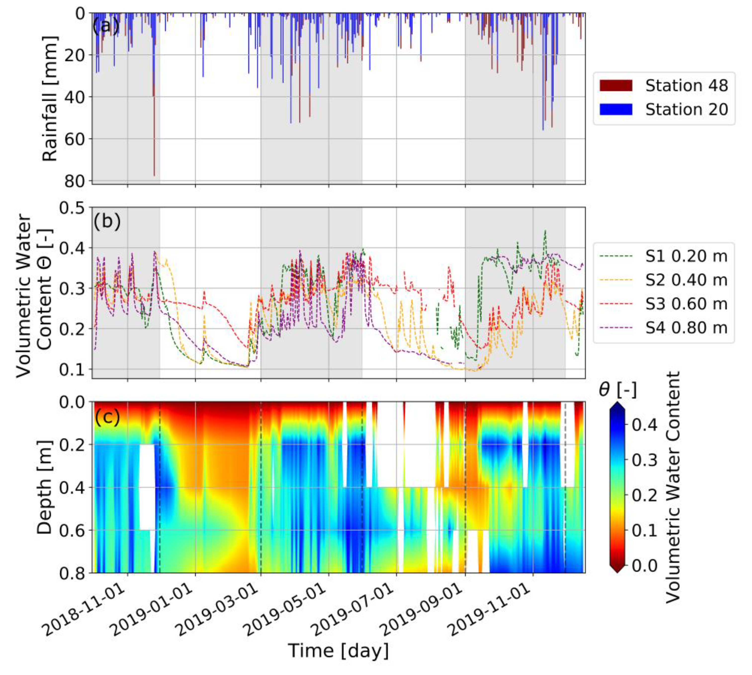
Figure 8 illustrates the behavior of soil moisture, showing the time evolution of measurements at four different depths. Soils at the study site have clay textures and a high content of rock blocks at depth [17]. In general, we observed a relatively rapid response of the soil moisture to the rainfall events (within a day) for all installed sensors. For the shallowest (0.2 m), the soil is usually above field capacity (68% of the year); during the dry seasons, soil moisture approaches the wilting point. Rainfall events > 40 mm/day favor rapid soil saturation. At 0.6 m below the surface, the soil mostly remains very wet year-round (Figure 8b,c), rapidly reaching the saturation point. In general, sensors at 0.4 and 0.8 m depths show the best relation for dry and wet periods (Figure 8b).
The recorded values of soil moisture are consistent with the behavior of the water table, which responds rapidly to precipitation and remains at shallow depths (<0.4 m) for most of the year, favoring the capillarity effects in the soil. Thus, the combination of high moisture values during most of the year and a perched water table very close to the surface, favors the rapid hydrological response in periods of high precipitation and facilitates the rapid saturation as a function of the volume and periodicity of precipitation.
4.3. Measurement of Movement
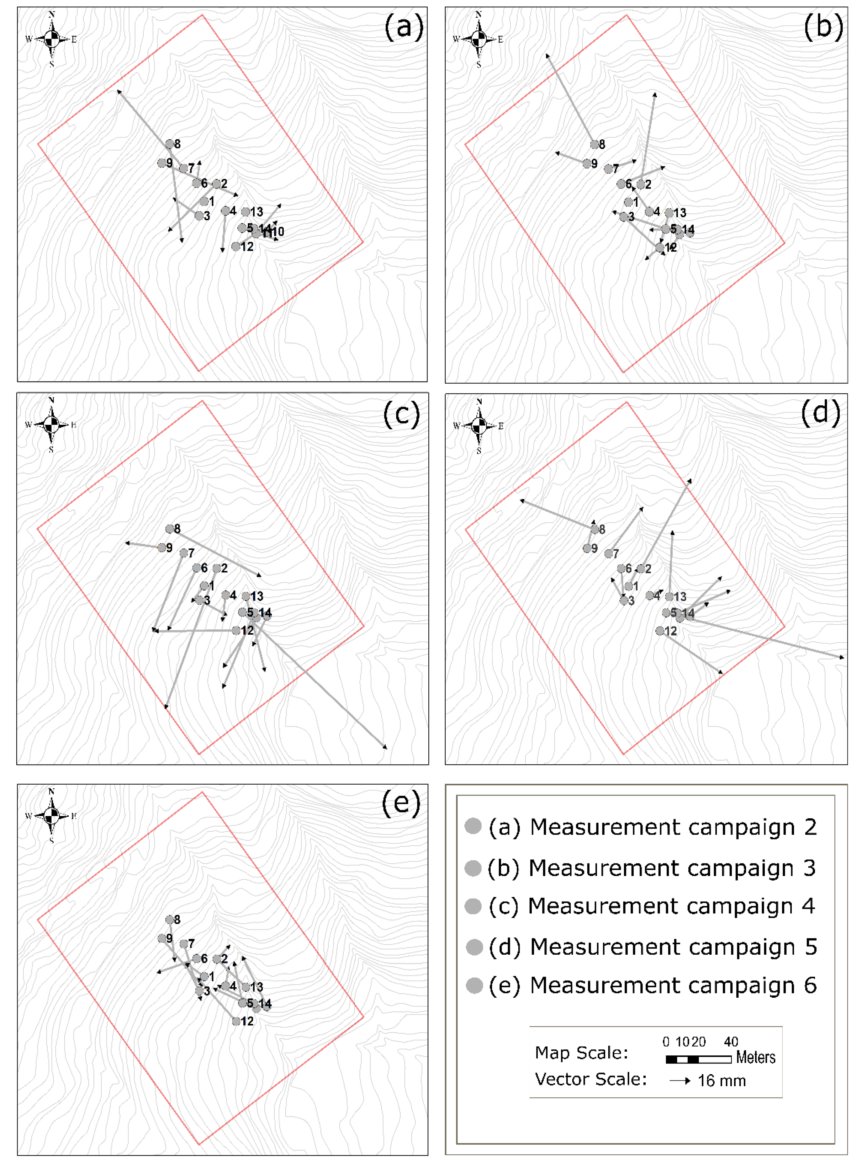
To estimate displacement magnitudes, we calculated the difference in position of the survey points between two consecutive measurements during each field campaign; the resulting vectors are shown in Figure 9. As the positions are relative to a point that is also moving, they cannot be interpreted as absolute positions and should only be taken as a first order result with the intention of estimating the short term evolution of the displacement. The survey observations yielded displacements between consecutive campaigns ranging from 15 to 204 mm. Results indicate that the smallest displacement magnitudes (in terms of mean values) occurred between November and December (campaign 6, mid-December, Figure 9e) and the largest displacements occurred between September and October (campaign 4, mid-October, Figure 9c). The spatial distribution of displacement does not show a specific pattern, and it seems like the maxima and minima of the vectors occur randomly.
It is noteworthy that in some cases, the displacement apparently occurs in a direction opposite to the prevailing slope gradient (Figure 9). This may be due to the fact that the motions are relative to a moving point and to counter-slope-wise rotations of the survey milestones. During campaign 4, the one with the largest mean displacement, only 2 out of 13 vectors have a component opposite to the slope gradient (Figure 9c); for campaign 6, which is associated with the shortest mean displacement, nine (9) vectors have a component opposite to the slope gradient (Figure 9e). This suggests that, in spite of the limitations, we are roughly capturing the downslope motion of the soil and that these displacement measurements are providing us with valuable preliminary information.
5. Discussion
The contributions of shallow groundwater to the soil water balance, evapotranspiration, plants, and ecosystems have been extensively studied and documented [38,39,40,41]. In our case, after measuring moisture for several months and at least two cycles of dry-wet time periods, we can identify an udic moisture regime, as there are horizons in the soil that remain wet all year, and even during the dry periods are nearly at field capacity. It is clear for measurements 0.6 m below the surface, the volumetric water content remains relatively high during the dry seasons. Additionally, the soil profile takes from two weeks to a month to reach a near saturation state after the beginning of the rainy season. This behavior is consistent with the observations of fluctuations in the water table, which remains near the surface for most of the year, supported by the presence of hydrophytes and evidence of redox features in the soil profile [17].
Based on a compilation of landslides near our study site, evidence exists that the first rainfall maximum of the year (during March–May) recharges the soils, so that during the second rainy season (September–November) the soil rapidly reaches saturation, initiating more landslides during this latter period [42]. Our data also suggest that the conditions of antecedent moisture in the soil determine the behavior of the soil water during the second annual rainy season; the high antecedent moisture between 0.4 and 0.6 m below the surface favors a rapid water table rise. Conversely, the water table decline during the dry season occurs slowly [43], as our data indicate that the levels in the piezometers take about 4 weeks to reach 0.6 m below the surface; during this season the capillarity plays an essential role in maintaining relatively high values of soil moisture, and the water table is highly controlled by textural discontinuities within the soil profile, which may be related to hydrologic discontinuities that create perched levels [17].
Percolation values measured in the deep lysimeter were systematically greater than those in the shallow one for both experimental plots during the rainy seasons, and it is common that percolation exceeds precipitation (Figure 7). These data indicate that subsurface lateral flow actively occurs at depths between 0.4 and 0.8 m; this is also consistent with the year-round shallow water table (most likely perched). Loaiza-Usuga et al. [17] present a more comprehensive description of this subsurface flow. Electrical resistivity surveys [17] suggest that meteoric water is concentrated in the uppermost 2 meters of the subsurface. Large rainfall events (>20 mm/day), in conjunction with near-field capacity antecedent moisture conditions, favor the saturation of the shallowest soil horizons and an increase in the surface runoff via saturation overland flow (Figure 7 and Figure 8). Similar situations have been reported by Corominas et al. [43] and Crosta [44] for mountain basins, where the soil parent materials determine porosity and the dynamics of water in the soil, which in turn may favor soil creep [43,45]. Therefore, we propose that the continuous subsurface downhill flow is exerting a quasi-permanent force upon the soil that actively contributes to creep.
The hummocky landscape at the study site is characterized by a series of mounds separated by irregular depressions, indicating a structure of independent blocks, which is consistent with very irregular and spatially discontinuous movement of the uppermost soil layers [18]. Expansion and contraction of the soil particles and the associated stresses are plausible processes to explain the heterogeneous movement of the soil that produces these geomorphic features; during years when the soil experiences drying, the effects of expansion and contraction on soil creep should be clearer. During our measurement period, even though the soil did not completely dry, there are variations in the water content which are linked to changes in the state of stress that contribute to soil movement.
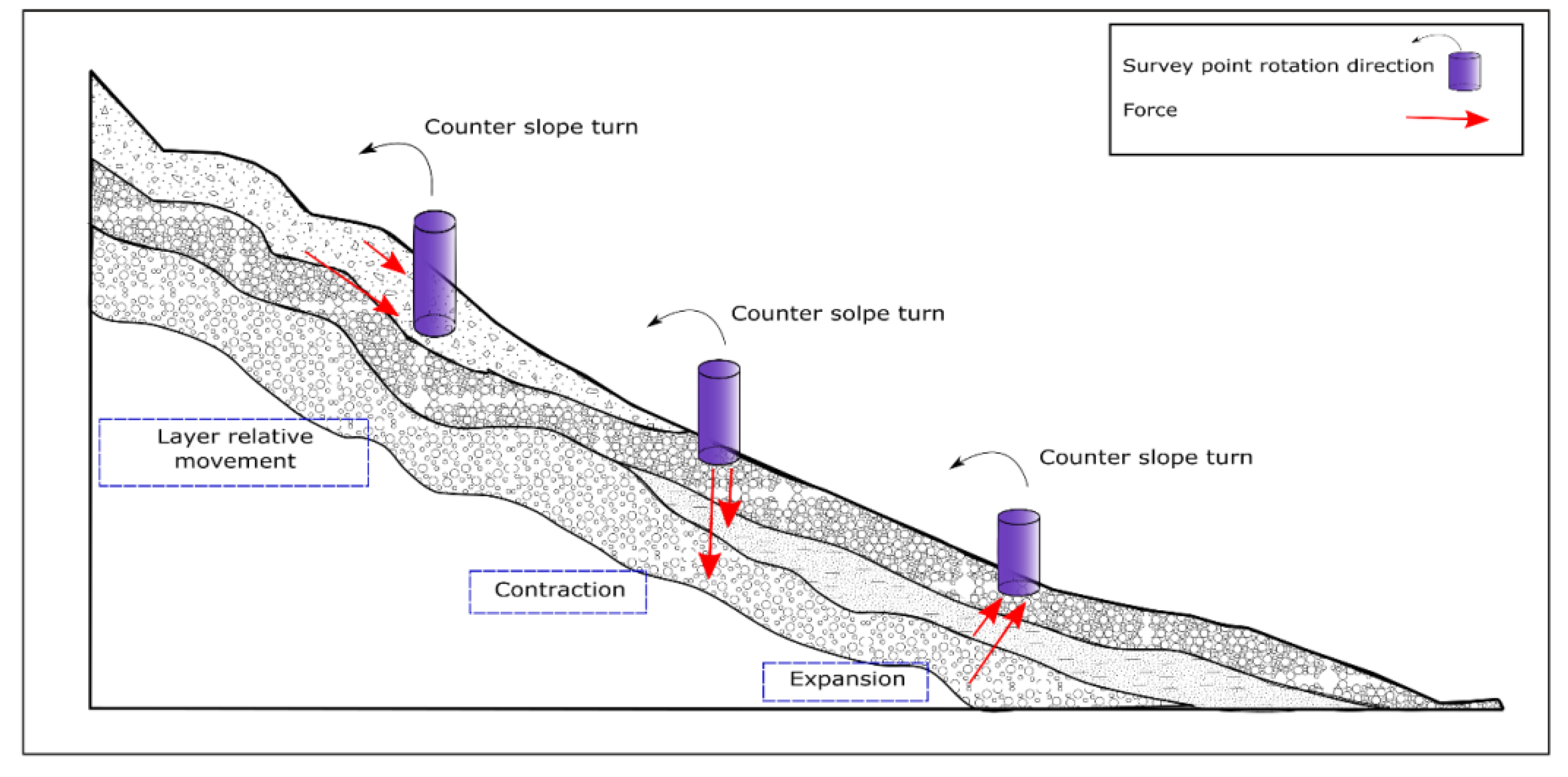
The results of the positioning measurements (Figure 9) indicate that slope creep movement is far from homogeneous; there exist apparent chaotic patterns with no clear trends. Even though this heterogeneous pattern arises because the positions were measured relative to a moving point, the results are consistent with the concept that there is not a single mechanism that drives soil creep, and rather a combination of factors such as expansion / contraction cycles, differential motion between layers, and effects of the subsurface flow acting at different depths, needs to be considered. Other studies note that short-term measurements of soil creep follow very heterogeneous and somewhat random patterns, and the net movement does not always occur in the direction of predominant slope gradient [46,47]; in our study site this was clearly the case. Additionally, in some cases, the movement (taken as the difference in positions between two consecutive survey campaigns) apparently occurs with a component in the upslope direction; as noted previously, this may be due to our measurements of relative positions with respect to a moving point. It is also clear that what we are measuring is not the position of the soil particle, but the position of a point on the cylinders used as milestones; torque on the 35 cm long cylinders, caused by the differential motion between soil layers, differential water push, or differential expansion / contraction stresses can generate this apparent upslope motion (Figure 10).
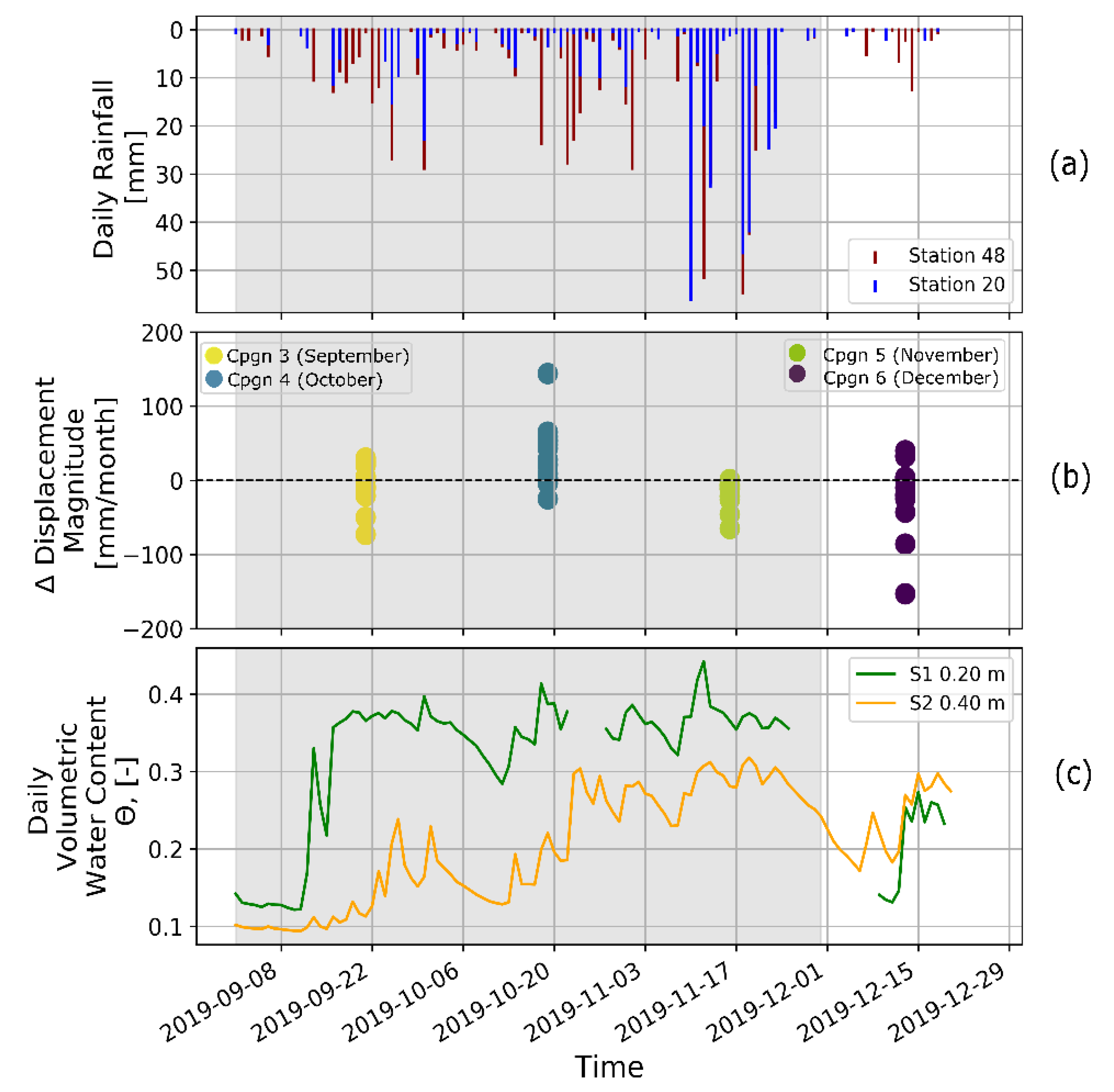
Aside from the fact that our positioning surveys do not necessarily measure soil motion, we interpret the change in the displacement magnitude (relative to the previous field campaign), regardless of the direction, as a first order indicator of creep rate. The change of magnitude of displacement is calculated by the difference in the displacement vector magnitude between two consecutive measurement periods. In Figure 11 it is shown that when using the positioning data from the mid-October field campaign, there is an increase in the magnitude of displacement relative to the one computed in the previous survey (mid-September); for the other campaigns (September, November and December), such movement decreases or remains approximately the same. This means that there is an increase in the displacement magnitude roughly between mid-September and mid-October in the middle of the rainy season (Figure 11b), the time during which water content in the soil approaches its maximum but fluctuates significantly in the upper layers of the soil (Figure 11c), changing the stress state and contributing to the movement. This correspondence between soil moisture fluctuations at a near-saturation state and the highest relative displacement magnitude, suggest that the expansion and contraction mechanism liked to soil wetting and drying, is playing a major role in soil creep.
The change in displacement magnitude reported for mid-September is given relative to the previous campaign, which was in July; during this period there is a transition from dry to wet seasons, with an associated increase in water content (Figure 11c); however, the displacement magnitude does not change significantly (Figure 11b). This is consistent with results by Crawford et al. [48] for a colluvial soil, where they found that the cumulative displacement decreased as the soil water content increased and approached saturation; the nature of this movement is different from the one we studied, but there is a similar response to the moisture change in terms of displacement rates. For the campaigns in mid-November and mid-December, the displacement magnitude predominantly decreases; between mid-October and mid-November, the soil moisture was at its highest, with smaller fluctuations compared with the previous period (mid-September–mid-October, Figure 11c). The relatively stable high-water content, in conjunction with the subsequent development of a more compact topsoil and a dense root system, may determine the decrease in the displacement rate [49]. During the time interval between mid-November and mid-December the dry season is established and the water content in the upper soil layers decrease (Figure 11c), consistent with stabilization as the drying occurs [48].
Unfortunately, the time window of our measurements is very limited and this is only a rather rough order estimate of what can occur at monthly time scales; to better address the role of the wetting / drying (expansion / contraction) processes in soil creep in our study site, a longer term positioning study should be continued. However, our data suggest that an increase in the displacement magnitude is related to fluctuations in the soil water content during a period of high pore pressure, and other factors, such as contrasting properties in between different soil layers and the forces exerted by subsurface lateral flow that contribute to the slow downhill movement of soil.
6. Summary and Conclusions
Different pieces of evidence indicate that soils are creeping in many locations on the western slope of the Medellín–Aburrá Valley, in the northern Andes of Colombia. The humid weather and the steep slopes make soil creep and landslides common in the area. We selected a monitoring site to improve our understanding of the creep phenomenon and to assess its relationship with the soil hydrology. We found a soil with significant vertical variations in texture and structure, which favor relative displacements in between different soil layers. The first 2 meters below the surface have a high-water content, resulting from perched water tables. We found sufficient evidence of active subsurface flow in the shallow subsurface (within the first 80 cm); forces exerted by this flow upon the soil particles are likely contributing to soil creep movement.
It is known that the effects of soil particle expansion and contraction, as a result of cycles of wetting and drying, are one of the main driving mechanisms of soil creep; this suggests a strong link between soil hydrology and its displacement. Therefore, we conducted a series of positioning surveys at the study site to elucidate this relationship. We observed that the relative displacement magnitudes and their changes were at their maxima between mid-September and mid-October, by the middle of the rainy season, so we infer that the effects of expansion / contraction seem to be more significant in terms of creep rate when changes in water content occur within a wet period, during which the soil is nearly saturated. In other words, our results suggest that changes in soil moisture during the rainy season play an essential role in favoring the slow downhill motion of the soil particles.
Supplementary Materials
The following are available online at https://www.mdpi.com/2076-3263/10/11/472/s1, Table S1:Basic statistics for runoff and percolation data measurements. Table S2: Basic statistics for the piezometric data measurements. Table S3: Basic statistics for net movements of the alti-planimetric surveys.
Author Contributions
Conceptualization, experiment designs, writing—review and editing were conducted by A.P.-P., G.M., J.C.L.-Ú., J.H.C.-A., L.I.A.-V., and R.C.S.; A.P.-P. performed the hydrological measurements and data processing; A.P.-P; J.H.C.-A. made the initial characterization of the study area. All authors have read and agreed to the published version of the manuscript.
Funding
This research received no external funding.
Acknowledgments
We would like to thank the students of the undergraduate program in Environmental Engineering at the National University of Colombia at Medellín for their help and participation during the measurements and field observations. The Area Curricular de Medio Ambiente (direction of the curricular programs in Environmental Sciences and Engineering) helped us with some resources to finish the experimental procedures. We also thank the Early Warning System of Medellín and the Aburrá Valley (SIATA, by its acronym in Spanish) for providing us with the precipitation time series.
Conflicts of Interest
The authors declare no conflict of interest.
References
- Aristizábal, E.; Roser, B.; Yokota, S. Tropical chemical weathering of hillslope deposits and bedrock source in the Aburrá Valley, northern Colombian Andes. Eng. Geol. 2005, 81, 389–406. [Google Scholar] [CrossRef]
- Echeverri, A.; Vélez, A.E.; Werthmann, C. Re Habitar la Ladera: Operaciones en Áreas de Riesgo y Asentamiento Precario en Medellín; Urbam (Centro de Estudios Urbanos y Ambientales—Universidad EAFIT): Medellín, Colombia; Harvard Design School: Cambridge, Mass, USA, 2012; pp. 1–70. [Google Scholar]
- Aristizábal, E.; Gómez, J. Inventario de emergencias y desastres en el Valle de Aburrá. Originados por fenómenos naturales y antrópicos en el periodo 1880–2007. Gestión y Ambiente 2007, 10, 17–30. [Google Scholar]
- García Londoño, C. Estado del conocimiento de los depósitos de vertiente del Valle de Aburrá. Boletín de Ciencias de la Tierra 2006, 19, 1–10. [Google Scholar]
- Loaiza-Úsuga, J.C.; Pauwels, V.R.N. Utilización de sensores de humedad para la determinación del contenido de humedad del suelo (Ecuaciones de Calibración). Suelos Ecuat. 2008, 38, 24–33. [Google Scholar]
- Pawlik, Ł.; Šamonil, P. Soil creep: The driving factors, evidence and significance for biogeomorphic and pedogenic domains and systems—A critical literature review. Earth-Sci. Rev. 2018, 178, 257–278. [Google Scholar] [CrossRef]
- Sidle, R.; Ochiai, H. Landslides: Processes, Prediction, and Land Use; America Geophysical Union, Water Resources Monograph No. 18: Washington, DC, USA, 2006; p. 312. [Google Scholar]
- Bayer, B.; Simoni, A.; Mulas, M.; Corsini, A.; Schmidt, D. Deformation responses of slow moving landslides to seasonal rainfall in the Northern Apennines, measured by InSAR. Geomorphology 2018, 308, 293–306. [Google Scholar] [CrossRef]
- Handwerger, A.L.; Roering, J.J.; Schmidt, D.A. Controls on the seasonal deformation of slow-moving landslides. Earth Planet. Sci. Lett. 2013, 377-378, 239–247. [Google Scholar] [CrossRef]
- Giovanni, C.; Frattini, P. Rainfall-induced landslides and debris flows. Int. Food Res. J. 2008, 22, 473–477. [Google Scholar] [CrossRef]
- Aristizábal, E.; Martínez, H.; Vélez, J.I. Una revisión sobre el estudio de movimientos en masa detonados por lluvias. Rev. de La Acad. Colomb. de Cienc. 2010, 34, 209–227. [Google Scholar]
- Rodríguez-Iturbe, I.; Porporato, A. Ecohydrology of Water-Controlled Ecosystems: Soil Moisture and Plant Dynamics, 1st ed.; Cambridge University Press: Cambridge, UK, 2005; pp. 1–464. [Google Scholar] [CrossRef]
- Malik, I.; Wistuba, M.; Migoń, P.; Fajer, M. Activity of slow-moving landslides recorded in eccentric tree rings of Norway spruce trees (Picea Abies Karst.)—An example from the kamienne MTS. (Sudetes MTS., Central Europe). Geochronometria 2016, 43, 24–37. [Google Scholar] [CrossRef] [Green Version]
- Šilhán, K. Dendrogeomorphic chronologies of landslides: Dating of true slide movements? Earth Surf. Process. Landf. 2017, 42, 2109–2118. [Google Scholar] [CrossRef]
- Gariano, S.L.; Guzzetti, F. Landslides in a changing climate. Earth-Sci. Rev. 2016, 162, 227–252. [Google Scholar] [CrossRef] [Green Version]
- Sidle, R.C.; Bogaard, T.A. Dynamic earth system and ecological controls of rainfall-initiated landslides. Earth-Sci. Rev. 2016, 159, 275–291. [Google Scholar] [CrossRef]
- Loaiza-Úsuga, J.C.; Monsalve, G.; Pertuz-Paz, A.; Arce-Monsalve, L.; Sanín, M.; Ramirez-Hoyos, L.F.; Sidle, R.C. Unraveling the Dynamics of a Creeping Slope in Northwestern Colombia: Hydrological Variables, and Geoelectrical and Seismic Signatures. Water 2018, 10, 1498. [Google Scholar] [CrossRef] [Green Version]
- Young, A. Soil movement by denudational processes on slopes. Nature 1960, 188, 120–122. [Google Scholar] [CrossRef]
- Gravenor, C.P.; Kupsch, W.O. Ice-Disintegration Features in Western Canada. J. Geol. 1959, 67, 48–64. [Google Scholar] [CrossRef]
- Wilding, L.P.; Smeck, N.E.; Hall, G.F. Pedogenesis and Soil Taxonomy, I. Concepts and Interactions, 1st ed.; Elsevier Science: Amsterdam, The Netherlands, 1983; Volume 11A, pp. 1–302. [Google Scholar]
- Pennock, D.J.; Zebarth, B.J.; De Jong, E. Landform classification and soil distribution in hummocky terrain, Saskatchewan, Canada. Geoderma 1987, 40, 297–315. [Google Scholar] [CrossRef]
- Soil Survey Staff–SSS. Keys to Soil Taxonomy, 12th ed.; Soil Survey Staff (SSS), United States Department of Agriculture, Natural Resources Conservation Service: Washington, DC, USA, 2014; pp. 1–372. [Google Scholar]
- Instituto Geográfico Agustín Codazzi—IGAC. Estudio General de Suelos y Zonificación de Tierras. Departamento de Antioquia. Tomo 2; Instituto Geografico Agustin Codazzi (IGAC): Bogotá, Colombia, 2007; pp. 664–672. [Google Scholar]
- Lindbo, D.L.; Stolt, M.H.; Vepraskas, M.J. Redoximorphic features. In Interpretation of Micromorphological Features of Soils and Regoliths; Stoops, G., Marcelino, V., Mees, F., Eds.; Elsevier: Amsterdam, The Netherlands, 2010; pp. 129–147. [Google Scholar]
- Espinal, S. Geografia Ecológica de Antioquia. Zonas de Vida; EALON—Universidad Nacional de Colombia: Medellin, Colombia, 1992; pp. 1–146. [Google Scholar]
- Heimsath, A.M.; Jungers, M.C. Processes, Transport, Deposition, and Landforms: Quantifying Creep. Treatise Geomorphol. 2013, 7, 138–151. [Google Scholar] [CrossRef]
- Carson, M.A.; Kirkby, M.J. Hillslope form and Process; Cambridge University Press: Cambridge, UK, 1972; pp. 1–476. [Google Scholar]
- Huggett, R. Fundamentals of Geomorphology, 4th ed.; Routledge: London, UK, 2016; pp. 1–578. [Google Scholar]
- Kirkby, M.J. Measurement and theory of soil creep. J. Geol. 1967, 75, 359–378. [Google Scholar] [CrossRef]
- Saunders, I.; Young, A. Rates of surface processes on slopes, slope retreat and denudation. Earth Surf. Process. Landf. 1983, 8, 473–501. [Google Scholar] [CrossRef]
- Parizek, E.; Woodruff, J. A Clarification of the Definition and Classification of Soil Creep. J. Geol. 1957, 65, 653–657. [Google Scholar] [CrossRef]
- Bond, W. Soil Physical Methods for Estimating Recharge-Part. 3: Basics of Recharge and Discharge Series; CSIRO Publishing: Collingwood, Australia, 1998; pp. 1–21. [Google Scholar]
- Chu, J.; Low, B.K.; Choa, V. Soil Improvement: Prefabricated Vertical Drain Techniques; Thomson Learning Asia: Singapore, 2003; pp. 1–341. [Google Scholar]
- Twarakavi, N.K.; Šimůnek, J.; Schaap, M.G. Can texture-based classification optimally classify soils with respect to soil hydraulics? Water Resour. Res. 2010, 46, W01501, 1–11. [Google Scholar] [CrossRef] [Green Version]
- Twarakavi, N.K.; Sakai, M.; Šimůnek, J. An objective analysis of the dynamic nature of field capacity. Water Resour. Res. 2009, 45, W10410, 1–9. [Google Scholar] [CrossRef]
- Bedoya-Soto, J.M.; Aristizábal, E.; Carmona, A.M.; Poveda, G. Seasonal shift of the diurnal cycle of rainfall over Medellín’s valley, Central Andes of Colombia (1998–2005). Front. Earth Sci. 2019, 7, 92. [Google Scholar] [CrossRef]
- Vélez Otálvaro, M.V.; Vélez Upegui, J.I.; Carvajal Serna, L.F.; Ortiz Pimienta, C.; Cardona Orozco, Y.; Ramírez Rojas, M.I. CPA Ingeniería, Plan de Ordenación y Manejo de la Cuenca del río Aburra-Antioquia, Colombia; Universidad Nacional de Colombia: Medellín, Colombia, 2016; pp. 1–466. [Google Scholar]
- Gardner, W.R. Some steady state solutions of the unsaturated moisture flow equation with application to evaporation from a water table. Soil Sci. 1958, 85, 228–232. [Google Scholar] [CrossRef]
- Walker, J.; Bullen, F.; Williams, B.G. Ecohydrological changes in the Murray-Darling Basin: I. The number of trees cleared over two centuries. J. Appl. Ecol. 1993, 30, 265–273. [Google Scholar] [CrossRef]
- Vervoort, R.W.; van der Zee, R.W. Simulating the effect of capillary flux on the soil water balance in a stochastic ecohydrological framework. Water Resour. Res. 2008, 44, W08425. [Google Scholar] [CrossRef] [Green Version]
- ShokriKuehni, S.; Raaijmakers, B.; Kurz, T.; Or, D.; Helmig, R.; Shokri, N. Water Table Depth and Soil Salinization: From PoreScale Processes to FieldScale Responses. Water Resour. Res. 2020, 56. [Google Scholar] [CrossRef]
- Moreno, H.; Vélez, M.V.; Montoya, J.; Rhenals, R. La lluvia y los deslizamientos de tierra en Antioquia: Análisis de su ocurrencia en las escalas interanual, intra anual y diaria. Revista EIA 2006, 5, 59–69. [Google Scholar]
- Corominas, J.; Moya, J.; Ledesma, A.; Lloret, A.; Gili, J.A. Prediction of ground displacements and velocities from groundwater level changes at the Vallcebre landslide (Eastern Pyrenees, Spain). Landslides 2005, 2, 83–96. [Google Scholar] [CrossRef]
- Crosta, G. Regionalization of rainfall thresholds: An aid to landslide hazard evaluation. Environ. Geol. 1998, 35, 131–145. [Google Scholar] [CrossRef]
- Freeze, R. The Mechanism of Natural Ground-water Recharge and Discharge: 1. One-dimensional, Vertical, Unsteady, Unsaturated Flow above a Recharging or Discharging Groundwater Flow System. Water Resour. Res. 1969, 5, 153–171. [Google Scholar] [CrossRef]
- Finlayson, B. Field measurements of soil creep. Earth Surf. Process. Landf. 1981, 6, 35–48. [Google Scholar] [CrossRef]
- Imaizumi, F.; Sidle, R.C.; Togari-Ohta, A.; Shimamura, M. Temporal and spatial variation of infilling processes in a landslide scar in a steep mountainous region, Japan. Earth Surf. Process. Landf. 2015, 40, 642–653. [Google Scholar] [CrossRef]
- Crawford, M.M.; Bryson, L.S.; Woolery, E.W.; Wang, Z. Long-term landslide monitoring using soil-water relationships and electrical data to estimate suction stress. Eng. Geol. 2019, 251, 146–157. [Google Scholar] [CrossRef]
- Jahn, A. The soil creep on slopes in different altitudinal and ecological zones of Sudetes Mountains. Geogr. Ann. Ser. A Phys. Geogr. 1989, 71, 161–170. [Google Scholar] [CrossRef]
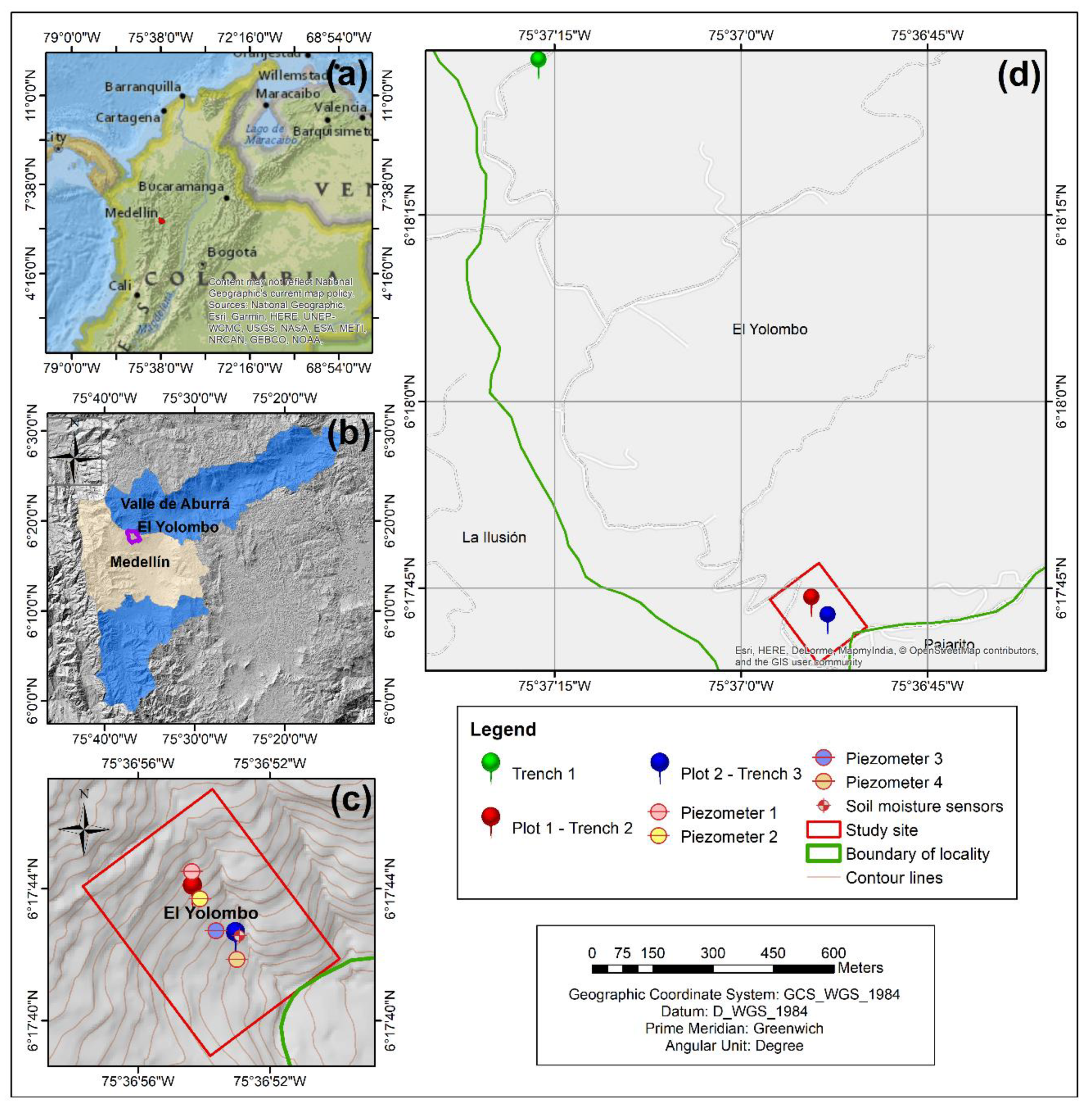
Figure 1.
Location of the study site: (a) The northwestern corner of South America and the Northern Andes; location of Medellín shown in red; (b) location of the study area relative to Medellín (gray) and the Aburrá Valley (blue); (c) monitoring site with the hydrological instrumentation; and (d) an expanded view including the location of trenches that we used to soil characterization; red box as in (c).

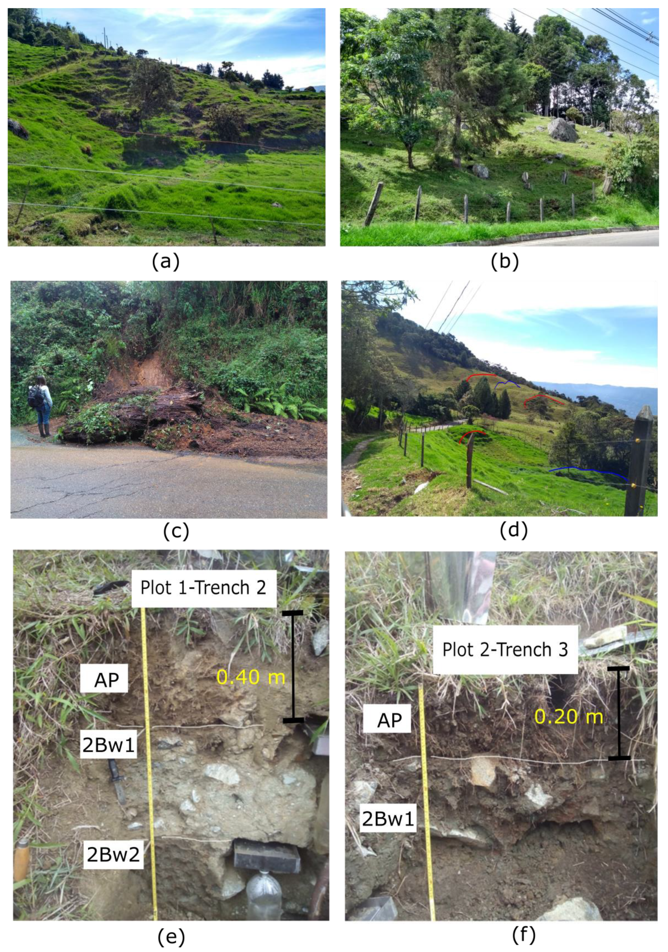
Figure 2.
General geomorphic, morphodynamic, and pedostratigraphic features around the study site: (a) terracettes; (b) terracettes, boulders, and mounds; (c) landslide on the road; (d) some scars (red) resulting from mobilized material, and signs of accumulated material (blue); (e) soil profiling at Plot 1; and (f) soil profiling at Plot 2; see Figure 1 for locations of plots and trenches.

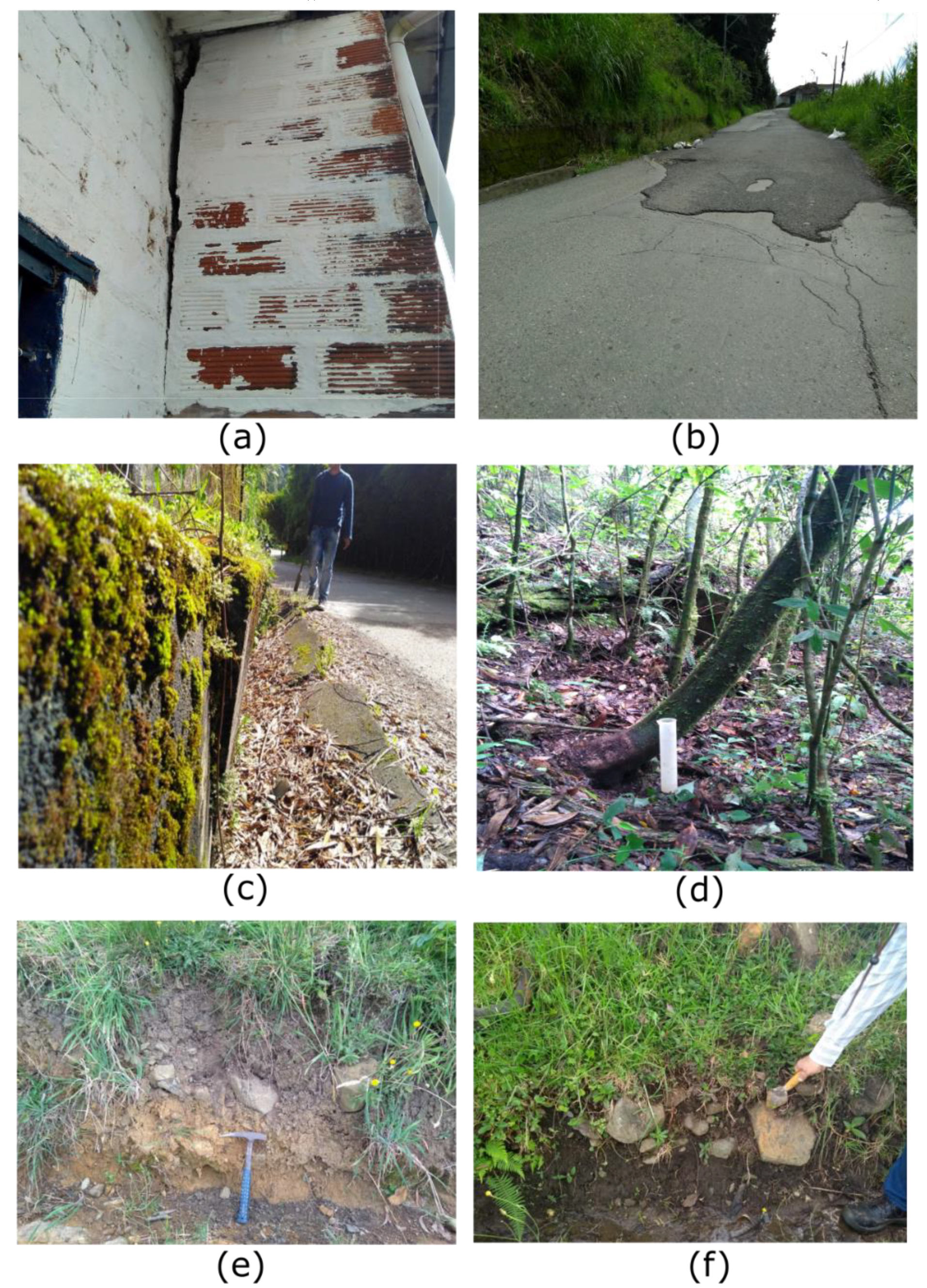
Figure 3.
Evidence of soil creep in the study area: (a) cracked walls; (b) cracks in roads; (c) broken retaining walls; (d) bent trees; (e) organic matter overlying the slope deposit; and (f) horizon of organic matter mixed with subangular rock blocks. The mass movement at our site was not classified as an earthflow since it implies a faster motion of the ground compared to creep, and therefore it would be more noticeable, while creep is nearly imperceptible [6,31]. Movement rates depend on the feedback among slope processes, pedogenesis, and biomorphic activity; together these generate complex morphometric characteristics, even at local scales [6]. Therefore, the activity of this phenomenon is not spatially uniform throughout the entire slope, causing the generation of the previously mentioned mounds and depressions, which agree with previous observations and reviews [6,8].

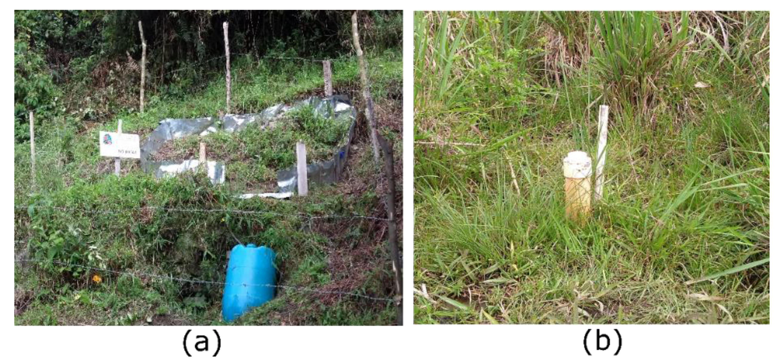
Figure 4.
Field instrumentation for hydrological measurements: (a) runoff plot; two zero-tension lysimeters were installed at different depths within the plots; and (b) one of the four piezometers installed along the slope.
Figure 4.
Field instrumentation for hydrological measurements: (a) runoff plot; two zero-tension lysimeters were installed at different depths within the plots; and (b) one of the four piezometers installed along the slope.

Figure 5.
Location of the survey points in the monitoring area. The triangle depicts the reference point for relative locations, and orange circles denote each survey point.
Figure 5.
Location of the survey points in the monitoring area. The triangle depicts the reference point for relative locations, and orange circles denote each survey point.

Figure 6.
Consolidated piezometer measurements. Daily rainfall is indicated at the top of diagrams, from two available gauges in the area (Stations 48 and 20). Gray shaded areas denote rainy seasons. Squares indicate water levels in each piezometer. Dashed line indicates the maximum depth reached by the piezometer. (a) piezometer 1; (b) piezometer 2; (c) piezometer 3; and (d) piezometer 4. See Figure 1 for piezometer location.

Figure 7.
Runoff and percolation measurements at the experimental plots. Gray shaded areas denote rainy seasons. (a) Daily rainfall from two rain gauges in the area; (b) runoff from plot 1; (c) percolation at two depths from plot 1 (indicated by the legend); (d) runoff from plot 2; and (e) percolation at two depths from plot 2 (indicated by the legend).

Figure 8.
Volumetric water content measurements with the sensors in Plot 2. Gray-shaded areas denote rainy seasons. (a) Daily rainfall from two rain gauges in the area; (b) time series of volumetric water content at each sensor. Legend indicates sensor depth; and (c) profile with the interpolation of volumetric water content in the soil profile.

Figure 9.
Displacement vectors between consecutive campaigns: (a) displacement campaign 2 with respect to campaign 1; (b) displacement campaign 3 with respect to campaign 2; (c) displacement campaign 4 with respect to campaign 3; (d) displacement campaign 5 with respect to campaign 4; and (e) displacement campaign 6 with respect to campaign 5.

Figure 10.
Schematic cartoon of the hillslope illustrating a possible cause for the obtained movements which are opposite to the slope gradient. Differential forces (red arrows) may act on the cylinders generating a torque that causes a counter slope turn, and therefore, an apparent upslope movement of the terrain. We illustrate the possible effects of differential downslope movements in between layers (left), differential vertical forces resulting from contraction (center), and differential surface–perpendicular forces resulting from expansion (right).

Figure 11.
Changes of displacement magnitude between consecutive campaigns. (a) daily rainfall from two rain gauges in the area; (b) changes of displacement magnitude for each survey point; and (c) time series of daily volumetric water content for the shallow sensors.
Figure 11.
Changes of displacement magnitude between consecutive campaigns. (a) daily rainfall from two rain gauges in the area; (b) changes of displacement magnitude for each survey point; and (c) time series of daily volumetric water content for the shallow sensors.


Table 1.
Main characteristics of the runoff plots.
| Plot 1 | Plot 2 | |
|---|---|---|
| Approximate slope (°) | 30 | 20 |
| Lysimeter 1 depth (cm) | 40 | 20 |
| Lysimeter 2 depth (cm) | 80 | 80 |
| Lysimeter 1 volume (L) | 20 | 30 |
| Lysimeter 2 volume (L) | 60 | 60 |
| Runoff tank volume (L) | 60 | 60 |
Table 2.
Frequency of soil moisture conditions according to measurements of Volumetric Water Content (VWC) at four sensors in Plot 2.
Table 2.
Frequency of soil moisture conditions according to measurements of Volumetric Water Content (VWC) at four sensors in Plot 2.
| Soil Moisture Condition | VWC Range (%) | Number of Data Points | Percentage |
|---|---|---|---|
| Sensor 1 (0.2 m depth) | |||
| Saturation | 0.39–0.45 | 5 | 1% |
| Partially saturated | 0.25–0.39 | 196 | 56% |
| Field capacity | 0.21–0.25 | 21 | 6% |
| Below Field capacity | 0.15–0.21 | 47 | 13% |
| Wilting point | 0.08–0.15 | 84 | 24% |
| Sensor 2 (0.4 m depth) | |||
| Saturation | 0.38–0.40 | 2 | 0% |
| Partially saturated | 0.36–0.38 | 3 | 1% |
| Field capacity | 0.34–0.36 | 16 | 4% |
| Below Field capacity | 0.19–0.34 | 233 | 55% |
| Wilting point | 0.17–0.19 | 19 | 4% |
| Hygroscopic point | 0.09–0.17 | 153 | 36% |
| Sensor 3 (0.6 m depth) | |||
| Saturation | 0.38–0.40 | 4 | 1% |
| Partially saturated | 0.36–0.38 | 22 | 5% |
| Field capacity | 0.34–0.36 | 21 | 5% |
| Below Field capacity | 0.19–0.34 | 338 | 81% |
| Wilting point | 0.17–0.19 | 13 | 3% |
| Hygroscopic point | 0.09–0.17 | 21 | 5% |
| Sensor 4 (0.8 m depth) | |||
| Saturation | 0.38–0.40 | 17 | 4% |
| Partially saturated | 0.36–0.38 | 61 | 15% |
| Field capacity | 0.34–0.36 | 34 | 8% |
| Below Field capacity | 0.19–0.34 | 136 | 32% |
| Wilting point | 0.17–0.19 | 36 | 9% |
| Hygroscopic point | 0.09–0.17 | 135 | 32% |
Table 3.
A chronology of the field campaigns.
| Campaign Number | Date |
|---|---|
| 1 | 06/15/2019 |
| 2 | 07/20/2019 |
| 3 | 09/21/2019 |
| 4 | 10/19/2019 |
| 5 | 11/15/2019 |
| 6 | 12/13/2019 |
Publisher’s Note: MDPI stays neutral with regard to jurisdictional claims in published maps and institutional affiliations. |
© 2020 by the authors. Licensee MDPI, Basel, Switzerland. This article is an open access article distributed under the terms and conditions of the Creative Commons Attribution (CC BY) license (http://creativecommons.org/licenses/by/4.0/).
Share and Cite
MDPI and ACS Style
Pertuz-Paz, A.; Monsalve, G.; Loaiza-Úsuga, J.C.; Caballero-Acosta, J.H.; Agudelo-Vélez, L.I.; Sidle, R.C. Linking Soil Hydrology and Creep: A Northern Andes Case. Geosciences 2020, 10, 472. https://doi.org/10.3390/geosciences10110472
AMA Style
Pertuz-Paz A, Monsalve G, Loaiza-Úsuga JC, Caballero-Acosta JH, Agudelo-Vélez LI, Sidle RC. Linking Soil Hydrology and Creep: A Northern Andes Case. Geosciences. 2020; 10(11):472. https://doi.org/10.3390/geosciences10110472
Chicago/Turabian StylePertuz-Paz, Aleen, Gaspar Monsalve, Juan Carlos Loaiza-Úsuga, José Humberto Caballero-Acosta, Laura Inés Agudelo-Vélez, and Roy C. Sidle. 2020. "Linking Soil Hydrology and Creep: A Northern Andes Case" Geosciences 10, no. 11: 472. https://doi.org/10.3390/geosciences10110472
Note that from the first issue of 2016, this journal uses article numbers instead of page numbers. See further details here.