Laboratory Studies Using Electrical Resistivity Tomography and Fiber Optic Techniques to Detect Seepage Zones in River Embankments

Abstract

We present the results of laboratory experiments on a down-scaled river levee constructed with clayey material collected from a river embankment where a permanent resistivity instrument has operated since 2015. To create potential seepages through the levee, two zones (5 × 4 cm and 10 × 2 cm) were filled with sand during the levee construction. Electrical resistivity tomography (ERT) technique and Fiber Bragg Grating (FBG) technology were used to study time-lapse variations due to seepage. The ERT profile was spread on the levee crest and the Wenner array with unit electrode spacing a = 3 cm was used. Six organic modified ceramics (ORMOCER) coated 250 μm-diameter fibers were deployed in different parts of the levee. Time-lapse measurements were performed for both techniques from the beginning of each experiment when water was added to the river side until the water was continuously exiting from the seepage zones. The results showed that ERT images could detect seepages from the early stages. Although with a short delay compared to ERT, fiber optic sensors also showed their ability to detect water infiltrations by measuring temperature changes. Both technologies being successful, a discussion about respective peculiarities and pros and cons is proposed to suggest some criteria in choosing the proper technique according to the specific needs.

1. Introduction

In the recent decade, hydrogeological risks have increasingly demanded development of proper solutions to be implemented in early warning alarming strategies. One of the most important and widely spread hydrogeological risks is the failure of earthen embankments that can happen on the slopes of roadways and railways, earthen dams, and river levees. Long-term monitoring systems should be developed and installed in risky areas to minimize the impacts of such failures. Electrical resistivity tomography (ERT) method is one of the most flexible geophysical techniques that is widely used in a variety of engineering and hydrogeological investigations, e.g., [1,2,3,4,5,6,7,8,9,10,11,12,13,14,15,16,17,18,19,20]. Having the capability of determining anomalous water saturation areas, as well as detecting seepage zones, the ERT method has been increasingly used to monitor the internal conditions of earthen embankments [21,22,23,24,25,26,27,28].

In order to monitor the integrity of river embankments, two customized ERT monitoring systems are in operation along two river embankments in Italy. ERT measurements with 48 electrodes (buried in 0.5 m-deep trenches) are supported by these systems, and the Wenner array was selected for these sites. The first pilot site was the levee of an irrigation canal in San Giacomo delle Segnate, northern Italy, where the unit electrode spacing a = 1 m was used [24]. The second pilot site was a critical section of the levee of Parma river in Colorno where the unit electrode spacing a = 2 m was used [21].

Although the ERT method is an efficient solution for long-term monitoring of the subsurface hydrogeological conditions, one drawback of this method is the dramatic increase in costs when lengths of more than a few hundred meters are to be studied. Such long lengths would demand longer cables and additional central units required to manage large numbers of electrodes that are necessary to achieve the desired lateral coverage. In this frame, fiber optic sensing technology can prove to be an interesting alternative for monitoring kilometers of earthen embankments. It offers the possibility of a permanent, real-time, and minimally invasive system that is able to provide multiple measurement points along the entire desired length only with a single fiber.

The feasibility of fiber optic sensors has been already demonstrated in some in-field experiments, e.g., [29] where optical fibers were deployed below the surface of the downstream slope, buried in a trench dug at the downstream toe of a levee, or directly embedded in geotextiles [29,30,31,32]. These studies have used distributed optical fiber sensing techniques such as Raman and Brillouin sensors. They could thus reconstruct temperature and deformation profiles along the entire length of the deployed sensing fiber (typically hundreds of meters) with the meter-spatial resolution. However, distinguishing “signatures” of seepage in acquired temperature data from anomalous strain field conditions within earthen embankments is still a challenging task, which requires considerable investigation to be clarified.

Integration of ERT and fiber optic sensing technologies can be an interesting solution to monitor the subsurface in a non-invasive manner, e.g., [17,33,34], and to better interpret the results of each individual method. In this paper, we present the results of integrating ERT and fiber optic techniques to monitor a down-scaled river levee constructed in a laboratory flume. Comparison of the results provided by ERT measurements and fiber optic sensors is helpful in evaluating the actual potential of each method in monitoring the internal conditions of levee structures and alarming the presence of seepage zones.

2. Laboratory Setup

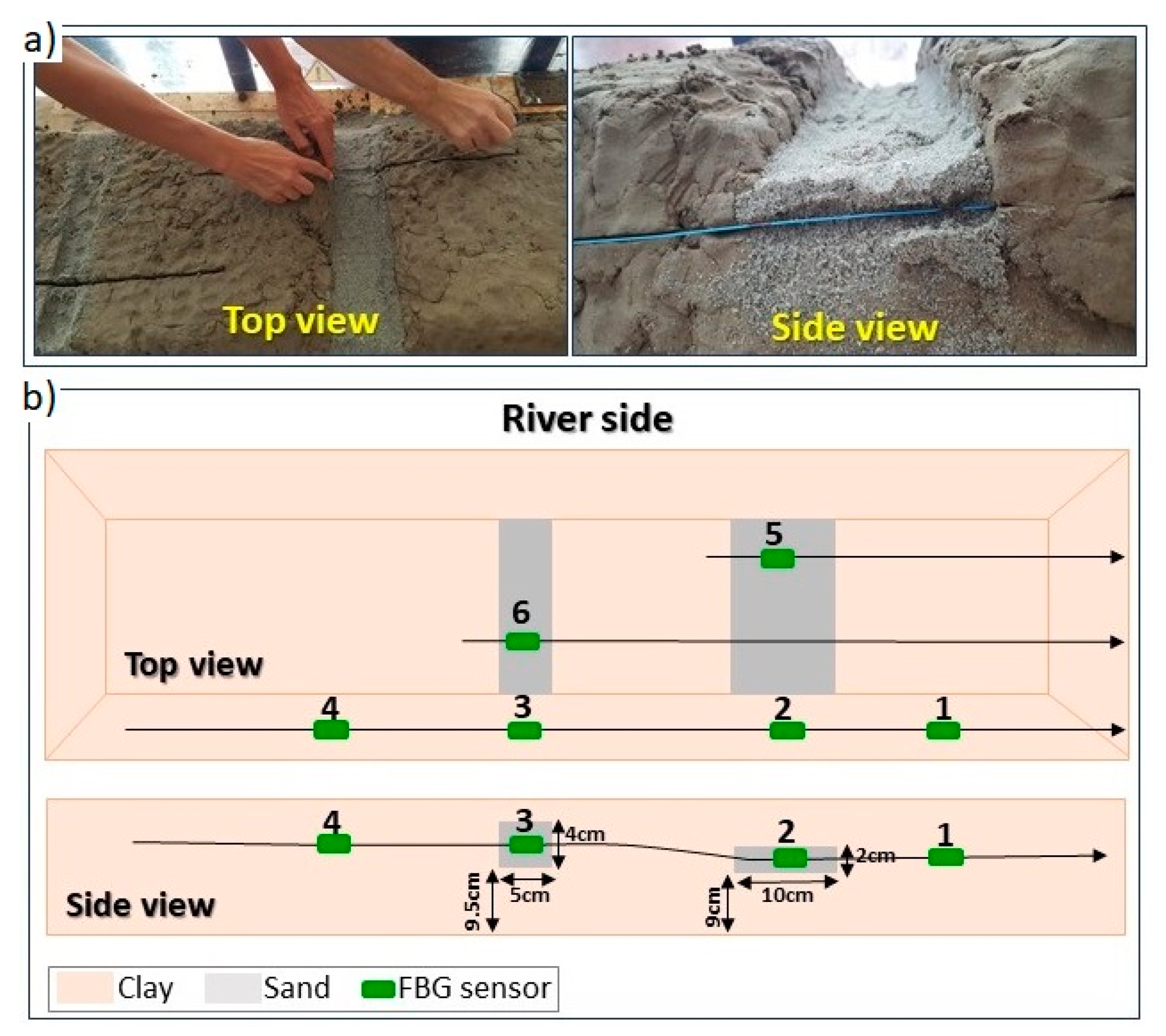
A down-scaled levee was constructed in a laboratory flume with transparent plexiglass walls (Figure 1). The material used to construct the down-scaled levee was the clay collected from the pilot site in San Giacomo delle Segnate where a permanent ERT system is in operation since 2015. The base size of the laboratory flume is 80 × 200 cm [35], and the plexiglass side walls are 50 cm high. In order to explore different ideas about the behavior of the San Giacomo delle Segnate levee body in response to internal/external variables for this pilot site, e.g., [33,36], the down-scaled levee was designed according to the geometry of the real site, applying a scaling factor of 1/12. The down-scaled levees were constructed with the top and bottom widths, respectively, equal to 28 cm and 55 cm. The levee height was 16 cm.

The main purpose of the experiments discussed in this paper was to compare the results of ERT and fiber optic techniques in detecting seepage zones inside levees. Therefore, in order to simulate seepages, two zones with the dimensions of 5 × 4 cm and 10 × 2 cm were filled with sand during levee construction (Figure 1a). In each experiment, the water level on the river side was gradually increased to the maximum height and it was kept constant until the end of the experiment. When arriving at the height of seepage zones, the water started leaking through these sandy zones and it could pass through the levee and continuously flow out from the opposite side (Figure 1b).

Two 24-channel cables assembled in-house and terminated with 48 stainless steel 2 cm-long mini electrodes [35] were used for ERT measurements. The Wenner electrode array with unit electrode spacing a = 3 cm was selected and the ERT profile was placed on top of the levee along its longitudinal axis (blue line in Figure 1b). Unfortunately, a cable failure occurred during some tests, which forced us to reduce the number of valid electrodes to 39. In all experiments, time-lapse ERT data were measured every 3 min using the high-speed option of Syscal Pro instrument (iris-instruments.com), which resulted in great time savings. The disadvantage was that every point of the apparent resistivity pseudosection was measured only once using this option, and thus, we do not have the possibility to perform statistical analysis that needs repeated measurements.

ERT measurements were integrated with fiber optic techniques to evaluate the feasibility of using the latter method to monitor the integrity of levee structures and to detect the presence of seepage zones. Since the meter-spatial resolution of Raman and Brillouin distributed fiber optic sensors [29,30,31,32] are suitable for 1:1-scale of field experiments and they are difficult to be exploited for a down-scaled setup that requires a spatial resolution of a few centimeters, Fiber Bragg Grating (FBG) technology was adopted in our laboratory experiments. FBGs are local gratings (length = 1 cm) inscribed at precise positions along the optical fiber [37], thus representing the ideal solution for monitoring small sections as in the current study. The results obtained in our investigation and the related considerations may, in any case, be extended (or considered valid) also for distributed fiber optic sensors regardless of the different sensitivity of distributed fiber optic sensors compared to FBGs that feature a high temperature and strain sensitivity of, respectively, 0.05 °C and 1 με [37].

Figure 2a illustrates the deployment of FBG sensors in different zones of the levee. In particular, six organic modified ceramics (ORMOCER) coated FBG along three 250 μm-diameter optical fibers, protected by a 900 μm plastic tube to guarantee mechanical strength, were deployed in different parts of the levee during its construction. The schematic plan of FBG sensors deployed in different parts of the levee is shown in Figure 2b. FBG 5 and FBG 2 were used to monitor the wider seepage zone, while FBG 6 and FBG 3 were used to monitor the narrower seepage zone. FBG 2 and FBG 3 were placed at seepage exits on the levee side that was not in contact with water, while FBG 5 and FBG 6 were placed inside the seepage zones, with FBG 5 being closer to the river side. Two further FBGs, FBG 1, and FBG 4 were buried in the clayey part of the levee, far away from the areas of potential infiltration. These two sensors were considered as a reference. It should be noted that FBGs are sensitive to both temperature and strain. Therefore, all FBGs were loosely inserted inside a 900 μm plastic tube to minimize their sensitivity to any strain-induced effect that may occur inside the levee as a consequence of water passage in the seepage. Therefore, we could analyze and compare mainly the thermal response of FBGs due to water infiltration.

We also used two GoPro Hero4 Session cameras to have additional tools for visual control of the experiments. The cameras were installed on the top frame of the laboratory flume so that the images recorded by these cameras could provide continuous monitoring from the top.

3. Data Processing and Results

Before inverting ERT datasets, they were cleaned for negative resistance values and extremely low injected currents. We usually remove bad quality data that have standard deviations larger than 2%, but since high-speed measurements did not provide the quality factor, this criterion could not be considered in this study. However, we performed some check measurements at random times using the stacking options to validate the high-speed measurements.

A further and important consideration before inverting the ERT datasets was to correct them for 3D effects. It is known that the 3D geometry can significantly disturb 2D ERT data measured along embankment structures like dams and river levees [38,39,40]. Since the level of water in the river side is an important parameter that can significantly change 3D effects [40], water level in the river side was continuously measured in our experiments. Moreover, the level of water on the other side of the levee was also measured continuously during the period when water was exiting from seepage zones. Apparent resistivity pseudosections measured at each time were then corrected for 3D effects using the approach discussed by Hojat et al. (2020) [36]. To do this, the 3D levee and its boundary conditions at different times were reconstructed in RES3DMODx64 (www.geotomosoft.com). It should be noted that the plexiglass sidewalls of the laboratory flume used in our experiments were resistive, and thus, they were also included in the 3D models, defined as lateral borders with high resistivity values similar to the air. The insulating base of the laboratory flume was also defined in synthetic 3D models as a highly resistive plane below the levee, extended in the vertical direction. The resistivity value used for the air, sidewalls and the base of the laboratory flume was 250,000 Ωm in synthetic models. The apparent resistivity pseudosections were then calculated for each model for the profile in the middle of the levee along its crest, corresponding to the position of the ERT profile measured in laboratory experiments. In the next step, 2D synthetic models were defined in RES2DMOD (www.geotomosoft.com) at each measurement time, and the apparent resistivity pseudosections were calculated for each model. To remove the 3D effects, the apparent resistivity values measured at the laboratory at each time were divided by the ratios of the apparent resistivity values calculated in RES3DMODx64 at that time divided by those calculated in RES2DMOD. This results in correcting the data for 3D effects as well as the effect of the insulating bottom of the laboratory flume. The remarkable advantages of this approach compared to a 3D inversion performed by including a priori information about the 3D geometry of the levee and the corresponding lateral boundary conditions plus a Neumann boundary corresponding to the insulating base of the laboratory flume [15] are that the inversion is much faster and more stable, being 2D rather than 3D. Readers interested in more details on this method are suggested to read Hojat et al. (2020) [36]. Having corrected all raw data based on the abovementioned criteria, time-lapse ERT datasets were then inverted in Res2dinvx64 (www.geotomosoft.com). Data outliers were filtered using the histograms of RMS error statistics available in RES2DINVx64.

The time-lapse inversion provided successive images of the resistivity values and thus, it showed how the subsurface was changing with time. The quality of these images was strongly dependent on weighting the data that was determined from error estimates [18]. In order to avoid the temporal smear, we used the high-speed acquisition option for our measurements to minimize the sampling time over which any single resistivity snapshot was completed [41]. The disadvantage of this option was that since the same measurements were not repeated, the data error could not be estimated from the standard deviation of the readings. The data error was neither available from reciprocal measurements in our experiments. Since the main objective of the time-lapse data analysis in our experiments was to explore how fast the response of ERT measurements is to the initiation of seepage phenomenon and to compare it with fiber optics, we gave priority to high-speed data acquisitions. However, since we have many datasets available, we could benefit from a couple of measurements acquired when no changes were expected, and we followed the methodology proposed by Robert et al. (2012) to set a cutoff value for the resistivity percentage change to separate real anomalies from artifacts caused by noise [20]. 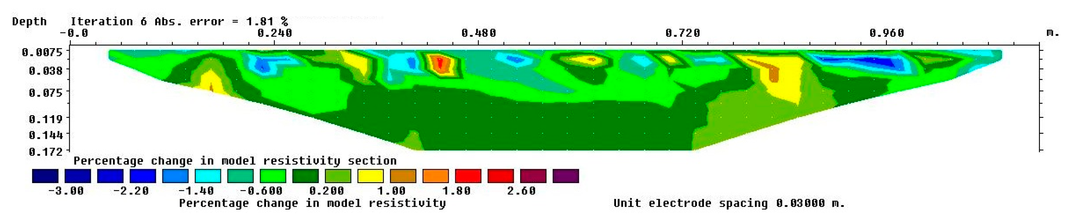Figure 3 illustrates an example of the percentage change in resistivity for two different measurements acquired at times when no changes were occurring. Note that these datasets were inverted in a time-lapse frame. We observed that the percentage change in resistivity is between −2.07 to 1.71%, which suggests that any resistivity change observed in our tests with percentage smaller than ±2% is not interpretable because it cannot be distinguished from the background noise artifacts.

We then selected the simultaneous time-lapse inversion method, and we set the smooth time-lapse inversion constrain in Res2dinvx64 (www.geotomosoft.com). We did not test other time-lapse inversion algorithms because the results with this approach were good enough in showing the expected changes on the inverted images. To better recognize changes in the internal condition of the levee structure, sections of the percentage change in resistivity values at different times were plotted. The simple difference between subsequential time-lapse data was suitable to underline small variations in resistivity related to water flow in our controlled laboratory experiments. It should be noted that when analyzing long-term monitoring data for more complex real field sites with un-controlled external variables and unknown internal processes, more detailed temporal analyses are required [26].

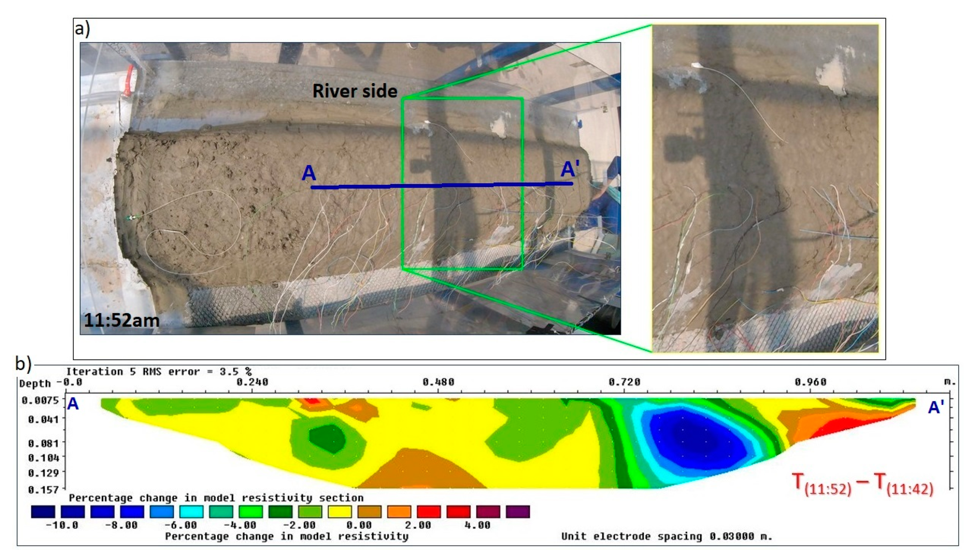
Figure 4a illustrates an example of GoPro pictures for one of the experiments at 11:52 a.m. when the water had already entered the 10 cm-wide seepage zone located at the horizontal distance 76 cm along the ERT line. At this time, water started entering the 5 cm-wide seepage zone located at the horizontal distance 33 cm along the ERT line. As can be recognized from the zoomed picture on the right side in Figure 4a, the water was not still exiting from the other side of the levee at this time, and thus, no visual evidence of seepage in a real case could be observed. Figure 4b presents the percentage change in resistivity distribution inside the levee body at 11:52 a.m. with that at 11:42 a.m. when the water height in the river side was below both seepage zones. We can observe that when the water had entered the wider seepage zone, the resistivity values of the levee body in this part were reduced about −10% compared to the time when this zone was dry. The very-early-stage entrance of water in the second zone was also evident, resulting in changes in resistivity values of about −2 to 3%. Note that such a small change slightly exceeds the defined noise level and we interpreted it as an anomaly in this test only because it is consistent with the expected anomaly. However, we could observe in the successive measurement that the percentage change in resistivity in this zone rapidly reached about −6%, which cannot be misinterpreted any more. This example is a typical illustration of how ERT monitoring is capable of detecting seepage zones at very early stages.

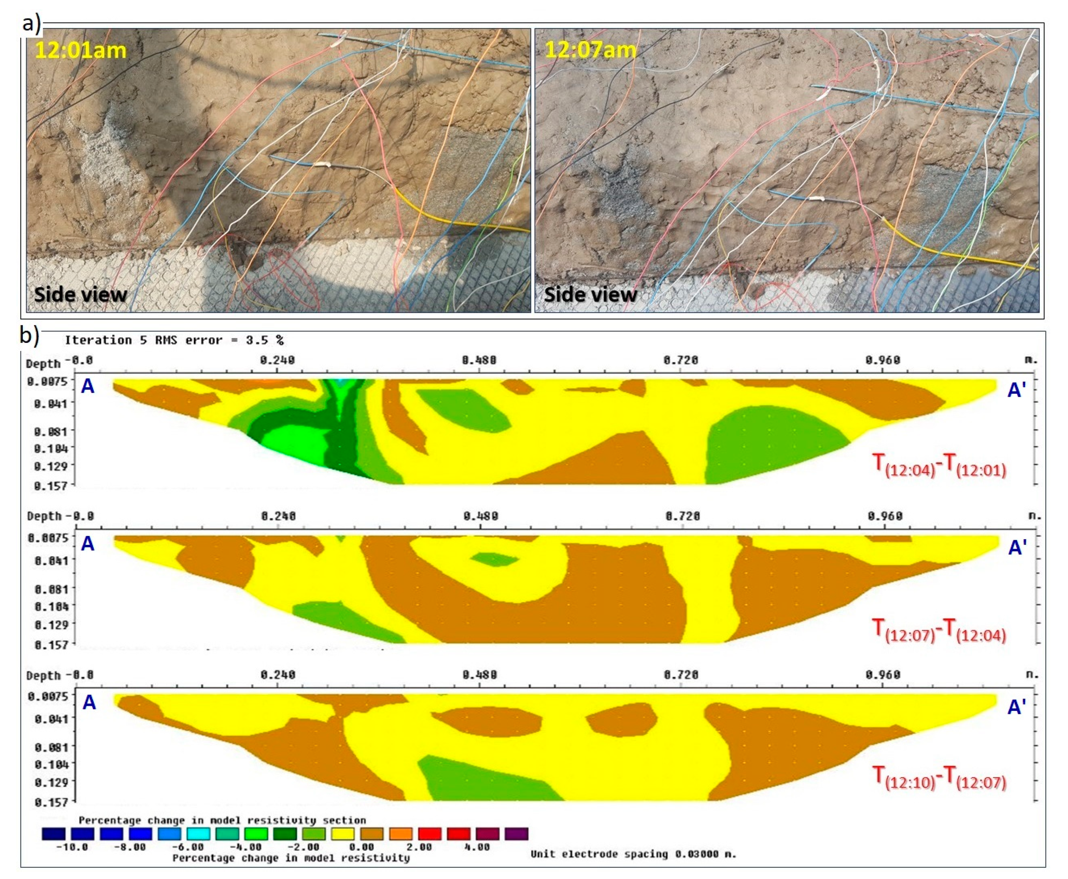
In all experiments, water was regularly injected in the river side and measurements were continued until water was continuously exiting from the other side. For the example experiment shown in Figure 4, the water flowed out from the 10 cm-wide seepage zone at 12:01 a.m. and from both seepage zones at 12:07 a.m. (Figure 5a). Figure 5b shows progressive percentage changes in resistivity values of the levee body from 12:01 a.m. until 12:10 a.m. It is interesting to note the first section in Figure 5b. This image shows the difference in resistivity values at 12:04 a.m. (when the water was not still exiting from the seepage zone on the left) with 12:01 a.m. (when the water is flowing out from the seepage zone on the right). This different situation can be recognized on the resistivity image, which shows a reduction in resistivity values for the left seepage zone while the percentage change in resistivity values for the seepage zone on the right is negligible because the water flow is stabilized in this zone and no significant change is occurring. The percentage changes in resistivity values for all parts of the second and third images shown in Figure 5b are around zero with magnitudes lower than ±2%, which is the expected background noise level. This is because these images show differences in the times when the water is continuously exiting from both zones and no further changes happened in the levee condition.

Figure 6 demonstrates the results obtained from the fiber optic sensors located inside and at exits of the two seepage zones. Figure 6a provides the temporal behavior of the local temperature measured by FBG 5, which is placed inside the wider seepage, closer to the river side. It can be noticed that just before 11:50 a.m., the rate of temperature increase slowed down and the trend was reversed at about 11:55 a.m. This indicates that the local temperature of the levee body (which was slowly warming up due to the presence of the sun beating on the levee) began to be reduced due to the passage of water that was a few degrees colder. The time period during which the slope change and a subsequent inversion occurred in temperature changes is well in agreement with the results obtained from ERT measurements that indicated the entering of water in the wider seepage zone at 11.52 a.m. (see Figure 4b). A similar transition is also visible in Figure 6b for the temperature profile recorded by FBG 6, which was located inside the narrower seepage zone that, according to direct observations as well as ERT data, was hosting water a couple of minutes after the wider seepage zone. In fact, a comparison of Figure 6b with Figure 6a shows that the temperature inversion for FBG 6 occurred a few minutes later compared to FBG 5. This delay was caused by several cooperating factors: (i) water arrived at the lower level of the narrower seepage two minutes later compared to the wider seepage because of the slightly different elevations of the two sand channels (Figure 2b), (ii) the two seepage channels had the same section area, but water arrived at the upper level of the narrower seepage much later compared to the wider seepage because of different thicknesses of the two seepage zones (Figure 2b), (iii) FBG 6 was placed farther from the river side compared to FBG 5 (Figure 2b).

Figure 6c,d show the temperature profiles recorded by FBG sensors located at the exits of the two seepage zones, on the levee side that is not in contact with water. It can be seen on these graphs that FBG 2 (placed at the exit of the wider zone, a few tens of centimeters farther from FBG 5) feels a temperature inversion due to the passage of water almost simultaneously with FBG 5 and much earlier than FBG 3. This is in agreement with the observation that water entered and fully covered the entrance of the wider seepage zone quite quickly, establishing a rapid water flow within the seepage channel; instead, the process of water entering and fully covering the entrance of the narrower seepage started with a delay and took a longer time, causing a slower water flow, also proved by the delay between temperature drops recorded by FBG 6 and FBG 3.

We can also notice that the temperature differences registered by FBG 2 and FBG 3 (located at the exits of the seepage zones) are around 6 degrees and 8 degrees, respectively, while FBG 5 and FBG 6 recorded lower temperature drops (about 3 degrees). This is because the laboratory flume and thus, the levee body, was not kept at a constant environment with a stable temperature, as also demonstrated by the rising temperature trend before water arrival. Indeed, the experiment was performed on a summer day outside the laboratory when the sunlight was heating the levee (see Figure 5a for example). This made the levee surface to be warmed up. FBG 2 and FBG 3 were deployed at the exits of the seepage zones and immediately below a few millimeters of sand, thus subjected to direct sun radiation. FBG 5 and FBG 6 were instead deployed inside these zones, and they were covered with a few centimeters of compacted clay that protected the sand channels from direct sun radiation. Therefore, the background temperature recorded by FBG 2 and FBG 3 was higher compared to FBG 5 and FBG 6, resulting in larger temperature drops when water arrived at the exits of the seepage channels.

A further consideration can be also made looking at the different behavior regarding the trend of the temperature inversion. Different rates of temperature changes observed for the two seepage zones show that the dynamics of the seepage flow in the narrow and wide seepage zones might be different. While sudden decreases in temperature are recorded by both sensors monitoring the narrower seepage zones (FBG 6 and FBG 3), we observe a rather gradual thermal process in the wider seepage zone reflected by FBG 5 and FBG 2. The complexity of the involved thermal and hydrogeological processes and the possible interference of strain effects induced by the arrival of water at fiber sensor locations would require the comparison of the observed phenomena with modeling results in order to discuss reliable interpretations. This is beyond the objective of the present work, which mainly focused on the comparison of ERT and fiber optic technologies as early warning systems for seepages. An exhaustive modeling would require the knowledge or the measurements of a number of thermal, geotechnical, and hydrogeological parameters needed to constrain the simulations [42].

4. Discussion

We presented the results of laboratory tests using ERT and fiber optic techniques to monitor seepage zones through a down-scaled river levee. The ERT method is increasingly used in monitoring hydrogeological risks thanks to its sensitivity to the variations of soil water saturation. The results of time-lapse ERT measurements showed a notable decrease in resistivity values as soon as the water enters seepage zones. The reduction trend in resistivity values continued until water was exiting from the other side, i.e., until a stable distribution of water within the levee was reached.

Despite proving to be an efficient solution for long term monitoring of hydrogeological risks, the ERT method demands increased costs as the desired length/area to be monitored is increased. This is due to the increased costs required for longer cables, larger number of electrodes, and additional central units. On the contrary, fiber optic sensing technology can be a cost-effective alternative for monitoring kilometers of lengths, offering the possibility to provide multiple measurement points along the entire desired length with a single fiber. The results of our tests showed the feasibility of this technology to detect water seepages thanks to temperature changes. Temperature profiles for different FBG sensors showed temperature trend inversions (due to water passage) occurring at times consistent with direct observations and with ERT results. ERT seems to be able to detect the occurrence of seepage at earlier stages compared to fiber sensors. This is due to different measurement principles, which in the ERT method is based on the injection of current from near-surface electrodes into large volumes of the levee body to produce a tomographic map of its resistivity, while the latter method requires the water seepage to approach the close vicinity of the fiber sensors. Therefore, tomographic images of ERT are affected by local variations in resistivity as soon as the water starts entering the seepage channel, while the sensing principle of the optical fibers requires the water to arrive at the position of the sensors. This was well highlighted in our results, where we observed that the fiber optic sensors deployed closer to the river side could provide alerts at the very early stage of water infiltration, well before the water would pass across the whole section of the levee. Optimum installations of fiber optics are thus very important to be implemented. Since such sensors are typically installed at the base of the levee opposite to the river side, an indication of the seeping water could be available only when it approaches the opposite side of the levee. The different measurement principles are also reflected in different installation requirements. Assuming that the objective is to detect any possible seepage occurring through the levee body, ERT can monitor the levee by installing a single line of electrodes along the main axis of the levee (typically buried at a depth of 40–50 cm). An added advantage of the ERT method is that the ERT spread is usually long enough so that the current can penetrate deeper than the height of the levee. Therefore, not only the levee body condition is adequately monitored in the resulting images, but the results can also detect the underseepage problem. On the contrary, fiber sensors need the physical contact with the seepage so that monitoring the full section of the levee body requires a spatially dense distribution of the fiber cable, which could be obtained by deploying a fiber zigzagging with a proper spacing between parallel lines (e.g., 1 m or less) on the levee side opposite to the river [30]. Although the cost of fiber optic is low, proper installation might become a challenging and invasive issue, especially when applying this technology to monitor the existing levees. However, fiber optic can be a very efficient and cost-effective solution for monitoring long distances of new embankments where the optical fiber can be easily installed within the levee body [43,44]. Finally, as mentioned in Section 2, fiber optic sensors are sensitive to both temperature changes and to deformations. To avoid any ambiguity in data interpretation for real in-field installations, sensing cables comprising both a tight fiber and a loose fiber are typically exploited to compensate for thermal effects on the tight fiber. This allows the correct recovery of any structural deformation of the levee caused by either water infiltrations or by the river water pressure and the correct recovery of temperature variations.

In this study, we were only interested in comparing the response of ERT and fiber optic techniques in detecting seepage channels through river levees. However, it is worth mentioning that using the calibrated empirical relationships between resistivity and water saturation [45], one important benefit in using the ERT method is the possibility to convert resistivity images into water saturation images, e.g., [26,35,36]. This is a significant point when we are interested in quantifying the water saturation in the levee to define thresholds for early warning alarms related to the instability of the structure. It should be noted that when aiming at converting the resistivity values into water content values for early-warning alarms, proper data processing must be applied to raw data. The most important factors to be corrected are the effect of the soil over buried electrodes, 3D effects, and temperature variations.

Standard geometrical factors for ERT measurements are defined for electrodes fixed on the ground surface. This means the complete reflection of the electric field at the surface. However, ERT layouts in long-term monitoring projects are usually buried below the surface at depths in the order of few tens of centimeters. This means that the current will also flow in the soil above the electrodes, and thus, a corrected geometrical factor must be considered for the apparent resistivity measurements. This correction can be applied using the image sources method [35,39,46].

As described in Section 3, we applied a method that corrects 2D ERT data for 3D effects before performing the 2D inversion. This is because a single 2D ERT layout deployed on the levee crest (which is the usual layout to monitor earthen embankments) would result in the distortions of 2D measured pseudosections due to 3D effects from the off-axis direction. The main advantage of the approach we used is reducing the computational time and memory required by a full 3D inversion. This is an important point in real-time monitoring projects where the inverse model is expected to be generated immediately after data acquisition. In order to accurately quantify 3D effects in real projects, a good knowledge of the material used for the construction of the levee is crucial. Moreover, variations of resistivity values in the levee during different seasons should be considered when calculating 3D effects for each period. In this paper, we were dealing with laboratory measurements and we knew the material used in different parts of the levee. We also measured the level of water on either side of the levee continuously. Therefore, we could properly construct synthetic models to estimate 3D effects. Helpful information about the proper model for real levees can be obtained by merging geophysical data with geotechnical data from laboratory analysis on core samples.

For what concerns the effect of temperature, daily variations of the air temperature would affect the soil temperature and accordingly the resistivity values down to 1 m [47,48,49]. It is also shown that long-term seasonal variations of the air temperature can affect the soil temperature down to more than 5 m [23,50]. Therefore, in order to correctly quantify the soil’s water content from resistivity data, ERT measurements acquired in a long-term monitoring period must be corrected, removing the external influence [26,51,52].

Time-lapse ERT monitoring is advantageous to study the dynamic effect of a particular parameter [53], mainly water content in hydrogeological studies. A very important issue in the time-lapse inversion of ERT data is to have an estimate of data error either from the standard deviation of repeated measurements or by using reciprocal measurements (www.geotomosoft.com). We used the high-speed acquisition option in our laboratory experiments, and thus, we didn’t have an estimate of data error. This might also be the case for many real studies where time constraints prevent measuring the noise estimation. In the study here, we used the methodology suggested by Robert et al. (2012) to estimate the background resistivity variations to prevent misinterpretation of the artifacts [20]. This is especially important in more complex real studies with more focus on quantitative analysis, and proper methodologies must be applied to estimate an interpretation threshold from the noise propagation during inversion, e.g., [14,19,20]. If using RES2DINVx64 for inverting the data, Loke (2018) suggests using the robust data constraint when adjusting the inversion parameters so that the effect of outliers in the data would be minimized on the inversion model (www.geotomosoft.com).

Fiber sensors could also present other benefits in terms of additional hydrogeological information that might be extracted from the analysis of the thermal behaviors of the sensors. This is an open issue that requires further investigations. In our future studies, a novel interrogation technique called Brillouin optical correlation domain analysis (BOCDA) [53] will be exploited, that with respect to the punctual information of FBGs, can recover the entire temperature and strain profiles along the deployed sensing fiber with centimetric-spatial resolution. Therefore, it allows an overall view on the behavior of the entire down-scaled levee during the seepage occurrence.

5. Conclusions

The results obtained in this work through the experimentation on a down-scaled clayey levee with two embedded sandy seepage zones showed how the timing of detecting water passage in seepage zones by the optical fiber sensors (easily indicated by a clear inversion of the temperature trend) was in good agreement with the ERT data. Although the ERT technique was capable of detecting seepage problems earlier compared to fiber optics, the results proved the feasibility of the fiber optic technique in monitoring the integrity of earthen embankments. Moreover, the results highlighted that deploying fiber optic sensors closer to the river side in future studies can provide alerts at the very onset of water infiltration, well before the water would cross the whole section of the levee and before ending in probable sudden damages. Optimum installations of fiber optics can be simply achieved when constructing new embankments, but their deployment might be limited in existing levees. On the contrary, since the most efficient layout for resistivity imaging of levees is to deploy the ERT profile on the levee crest along its longitudinal axis, installation of ERT systems is not seriously challenged, neither for the existing nor for new embankments. However, installation of ERT systems is seriously challenged when monitoring long sectors of levees is requested; this is because of the rapid increase in the costs due to the replication of the monitoring stations. Further pros and cons of the two techniques are reported in the discussion.