Development of a New Simulation Tool Coupling a 2D Finite Volume Overland Flow Model and a Drainage Network Model

Abstract

Numerical simulation of mixed flows combining free surface and pressurized flows is a practical tool to prevent possible flood situations in urban environments. When dealing with intense storm events, the limited capacity of the drainage network conduits can cause undesirable flooding situations. Computational simulation of the involved processes can lead to better management of the drainage network of urban areas. In particular, it is interesting to simultaneuously calculate the possible pressurization of the pipe network and the surface water dynamics in case of overflow. In this work, the coupling of two models is presented. The surface flow model is based on two-dimensional shallow water equations with which it is possible to solve the overland water dynamics as well as the transformation of rainfall into runoff through different submodels of infiltration. The underground drainage system assumes mostly free surface flow that can be pressurized in specific situations. The pipe network is modeled by means of one-dimensional sections coupled with the surface model in specific regions of the domain, such as drains or sewers. The numerical techniques considered for the resolution of both mathematical models are based on finite volume schemes with a first-order upwind discretization. The coupling of the models is verified using laboratory experimental data. Furthermore, the potential usefulness of the approach is demonstrated using real flooding data in a urban environment.

1. Introduction

Hydrologic/hydraulic modeling in urban environments is becoming a relevant tool to predict and evaluate the effects of storm events due to the failure of sewer systems. When this occurs, the flow within the pipe becomes pressurized and overflow appears in the linking elements as culverts or storage wells. The use of distributed models for surface flow simulations provides a more detailed computation of the spatial variations of the variables of interest. Within the bidimensional domain on the surface, this leads to detailed distributions of numerical results, such as the water depth or the flow discharge. This is of special relevance in abrupt terrain topographies or in urban areas where the buildings dramatically condition the flow direction.

It is traditionally accepted that the most accurate techniques for simulating surface flows of hydraulic interest are based on the solutions of the Shallow Water equations (SW) [1,2]. Numerical models based on SW have been developed for both 1D and 2D approaches [3,4,5,6]. However, the applicability of these models to any type of overland flow has a counterpoint in the usually high computational effort. Hence, the development of simplified models, capable of solving some particular situations with higher efficiency than the full SW model (e.g., Zero-Inertia model [7,8,9]), has widely been accepted.

One of the difficulties of numerical simulations of drainage networks is that they flow mostly under free surface conditions, but they are likely to become locally pressurized due to the limited storage capacity. Under these conditions, a complete drainage system model should be able to solve steady and transient flows under pressurized and unpressurized situations and the transition between both flows (mixed flows). Many of the models developed to study the propagation of hydraulic waves solve both systems of equations, e.g., [10]. For this purpose, a few numerical schemes derived from the Method of Characteristics (MOC) have been used. Other authors, e.g., references [10,11,12] developed numerical simulations by applying the 1D shallow water equations within a slim slot over the pipe (Preissmann slot method). An estimation of the conduit pressure can be obtained from the water level in the slot. This technique has been widely used to simulate local transitions between pressurized and shallow flows, but some stability problems have been reported [13] when simulating cases with abrupt transitions. This work is focused on the development of a coupled simulation model that is able to solve 2D overland flow in connection with a drainage system that can be exceptionally pressurized.

The non-linearity of the governing equations combined with the usually huge number of cells and hence, unknowns, in a complex problem implies a large amount of computing effort and time. There is an interest in developing efficient numerical methods. In general terms, numerical schemes used to solve time dependent problems can be classified in two groups attending to the time evaluation of the unknowns: explicit and implicit methods. Explicit schemes update the solution at every cell from the known values of the system at the current time, whereas implicit schemes generate a system of N equations with N unknowns, N being the number of computational cells multiplied by the number of variables to solve for each cell. Explicit schemes are restricted by numerical stability reasons. The advantage of using implicit schemes is that they are, in theory, unconditionally stable, even though they may be less accurate than explicit schemes for unsteady flows when using large time step sizes. A compromise is required between stability gain and accuracy loss on the results. Traditionally, this constitutes the main reason for using implicit methods in steady state computations. In these problems, the accuracy loss during the transient state is not so important, and the possibility of choosing a larger time step for the simulation often allows faster calculation of the steady state. In order to maximize the simulation efficiency by means of large time step sizes, some authors have applied implicit methods to SWE for solving 1D problems [14,15] and 2D problems [16,17,18,19,20,21].

There have been several previous works on 1D-2D dual drainage simulation models (coupling of 1D sewer network with 2D surface overland flow) in the literature [22,23,24,25,26,27,28,29]. In this kind of approach, the numerical model takes into account the flow through both surface and sewer system domains and establishes a communication between them at certain points, such as culverts or manholes.

The structure of the article is as follows: first, the mathematical models used to describe the flow dynamics are presented. The surface flow is formulated using the full (depth averaged) 2D shallow water equations. The drainage network flow is formulated using the full (cross sectional averaged) 1D shallow water equations together with the Preissmann slot strategy to account for local pressurization. Then, the proposed numerical approaches are presented. They are all finite volume techniques and can be divided into implicit and explicit schemes. The performance of the models is evaluated using experimental data from a laboratory test case and the results supplied for different scenarios are related to a real urban flow test case.

2. Model Representation

2.1. Surface Flow Model

Surface flow is modeled by means of the 2D full shallow-water equations [1], which can be expressed as follows:

$$\frac{\partial \mathbf{U}}{\partial t}+\frac{\partial \mathbf{F}\left(\mathbf{U}\right)}{\partial x}+\frac{\partial \mathbf{G}\left(\mathbf{U}\right)}{\partial y}=\mathbf{S}+\mathbf{H}+\mathbf{M},$$

(1)

where

$$\mathbf{U}={\left(h,q_x,q_y\right)}^T$$

(2)

are the vectors of conserved variables, where h represents the water depth and $q_x=hu$ and $q_y=hv$ are the unit discharges, with u and v being the depth averaged components of the velocity vector along the x and y coordinates, respectively. The fluxes of the conserved variables can be written as

$$\mathbf{F}={\left(q_x,\frac{q_x^2}{h}+\frac{1}{2}g{h}^2,\frac{q_x{q}_y}{h}\right)}^T,\mathbf{G}={\left(q_y,\frac{q_x{q}_y}{h},\frac{q_y^2}{h}+\frac{1}{2}g{h}^2\right)}^T,$$

(3)

where g is the acceleration due to gravity. The sources of (1) are split into three terms. The term $\mathbf{S}$ represents the friction losses, and it is defined as

$$\mathbf{S}={\left(0,-gh{S}_{fx},-gh{S}_{fy}\right)}^T,$$

(4)

where $S_{fx},S_{fy}$ are the friction slopes in the x and y directions, respectively, and are traditionally written in terms of the Manning’s roughness coefficient, n:

$$S_{fx}=\frac{n^{2}u\sqrt{u^2+v^2}}{h^{4/3}},S_{fy}=\frac{n^{2}v\sqrt{u^2+v^2}}{h^{4/3}}.$$

(5)

The term $\mathbf{H}$ accounts for the pressure force variation along the bottom in the x and y directions and can be formulated in terms of the bottom level z bed slopes:

$$\mathbf{H}={\left(0,-gh\frac{\partial z}{\partial x},-gh\frac{\partial z}{\partial y}\right)}^T.$$

(6)

The term $\mathbf{M}$ represents the mass sources/sinks due to rainfall/infiltration:

$$\mathbf{M}={\left(R-f+f_M,0,0\right)}^T,$$

(7)

where R is the local rainfall intensity, f is the local infiltration rate, and $f_M$ refers to a discharge per unit area of the manhole mouth. In order to take into account that there is a finite number of locations where the latter term participates, it has been formulated as follows:

$$f_M=\sum _j{I}_j(x,y)\frac{Q_{e,j}}{A_{M,j}},$$

(8)

where $I_j(x,y)=$ 1 if point $(x,y)$ corresponds to a manhole location, and it is nil otherwise. $Q_e$ is the exchange discharge between both domains, and $A_M$ is the area of the manhole.

2.2. Infiltration Law: Horton Model

Infiltration is the process by which surface water enters the soil. This process is mainly governed by two forces: gravity and capillarity action. In the present work, the Horton method was used. Horton’s infiltration model [30] suggests an exponential equation for modeling the soil infiltration capacity or maximum infiltration rate, $f_p$ (m/s):

$$f_p\left(t\right)=f_c+\left(f_0-f_c\right)e^{-kt},$$

(9)

where $f_0$ and $f_c$ are the initial and final infiltration capacities (m/s), respectively, and k represents the rate of decrease in the capacity ($s^{-1}$). The parameters $f_0$ and k have no clear physical basis, so they must be estimated from calibrating the model against experimental data. A good source for experimental values of these parameters for different types of soils can be found in Rawls et al. [31] and is summarized in ASCE [32].

Equation (9) assumes an unlimited water supply at the surface. This means that it has to be applied after surface ponding. It is important to highlight the difference between the infiltration capacity, $f_p$, and the infiltration rate, f. In absence of ponding surface water, if a rain event starting with a weak rainfall intensity ($R\le f_p$), then all the rain will completely infiltrate into the soil. On the other hand, if the rain intensity exceeds the soil infiltration capacity, the surface becomes ponded and Horton’s law (9) applies. Therefore,

$$f\left(t\right)=\left\{\begin{array}{cc}R\left(t\right)\hfill & \mathrm{if}R\left(t\right)\le f_p\left(t\right)\hfill \\ f_p\left(t\right)\hfill & \mathrm{if}R\left(t\right)>f_p\left(t\right).\hfill \end{array}\right.$$

(10)

The cumulative infiltration, $F\left(t\right)$, up to time t, can be calculated by integrating the infiltration capacity, f, as

$$F\left(t\right)={\int }_0^{t}f\left(t\right)dt=f_{c}t+\frac{f_0-f_c}{k}\left(1-e^{-kt}\right).$$

(11)

2.3. Discretization of the 2D Model

Assuming dominant advection, (1) can be classified as an hyperbolic system. In this case, the Jacobian matrix of the flux can be diagonalized and three real eigenvalues can be found. They are used to build the numerical contributions that update the flow variables and to control the numerical stability of the method. The system can be solved by an hybrid explicit/implicit, first-order, upwind finite volume scheme described in reference [2]. The wet/dry fronts are well tracked, providing stable solutions with a numerical mass error similar to machine accuracy. Adequate boundary conditions must be imposed, and the procedure also requieres initial condicions.

When using an explicit scheme, the time step size is limited for stability reasons [33]. The time step is dynamically chosen as follows:

$$\Delta t_{2D}=\mathrm{CFL}{\min }_{Mesh}(\Delta t_{i,w}),$$

(12)

where

$$\Delta t_{i,w}=\frac{\min (\Delta x_i^{\prime },\Delta x_j^{\prime })}{{\max }_{m=1,2,3}\left(\right|{\tilde{\lambda }}_w^m\left|\right)},\Delta x_i^{\prime }=\frac{S_i}{{\max }_{1,N_w}\left(l_w\right)}.$$

(13)

The numerical method is designed to work using any kind of mesh (unstructured triangular or structured rectangular). The convenience of using one or other is given by the specification of each problem. In case of using structured 2D meshes, the maximum CFL number for the explicit scheme is 1/2, whereas CFL = 1 is allowed for some unstructured triangular meshes [34]. On the other hand, implicit schemes benefit from theoretical unconditional stability. Hence, the CFL number becomes a multiplicative factor of the maximum time step allowed by the explicit scheme for stability reasons. The present formulation is well-balanced, that is, it ensures mass conservation and preserves the lake at rest property in the presence of source terms. It closely follows the results in reference [2].

2.4. Drainage System Model

It is generally accepted that unsteady open channel water flows can be simulated using the 1D shallow water or St. Venant equations. These equations represent mass and momentum conservation along the main direction of the flow and are a good description for most of the pipe-flow-kind problems. They can be written in a conservative form as follows:

$$\frac{\partial A}{\partial t}+\frac{\partial Q}{\partial x}=q_e$$

(14)

$$\frac{\partial Q}{\partial t}+\frac{\partial }{\partial x}\left(\frac{Q^2}{A}+g{I}_1\right)=g{I}_2+gA\left(S_0^{1D}-S_f^{1D}\right),$$

(15)

where A is the wetted cross section, Q is the discharge, $I_1$ represents the hydrostatic pressure force term, $q_e$ is the exchange discharge per unit length, and $I_2$ accounts for the pressures forces due to pipe width changes:

$$I_1={\int }_0^{h_p(x,t)}\left(h_p-\eta \right)b(x,\eta )d\eta$$

(16)

$$I_2={\int }_0^{h_p(x,t)}\left(h_p-\eta \right)\frac{\partial b(x,\eta )}{\partial x}d\eta$$

(17)

$$b=\frac{\partial A(x,\eta )}{\partial \eta }.$$

(18)

The remaining terms, $S_0^{1D}$ and $S_f^{1D}$, represent the bed slope and the energy grade line (defined in terms of the Manning roughness coefficient), respectively:

$$S_0^{1D}=-\frac{\partial z_p}{\partial x},S_f^{1D}=\frac{Q\left|Q\right|n_{1D}^2}{A^2{R}^{4/3}},$$

(19)

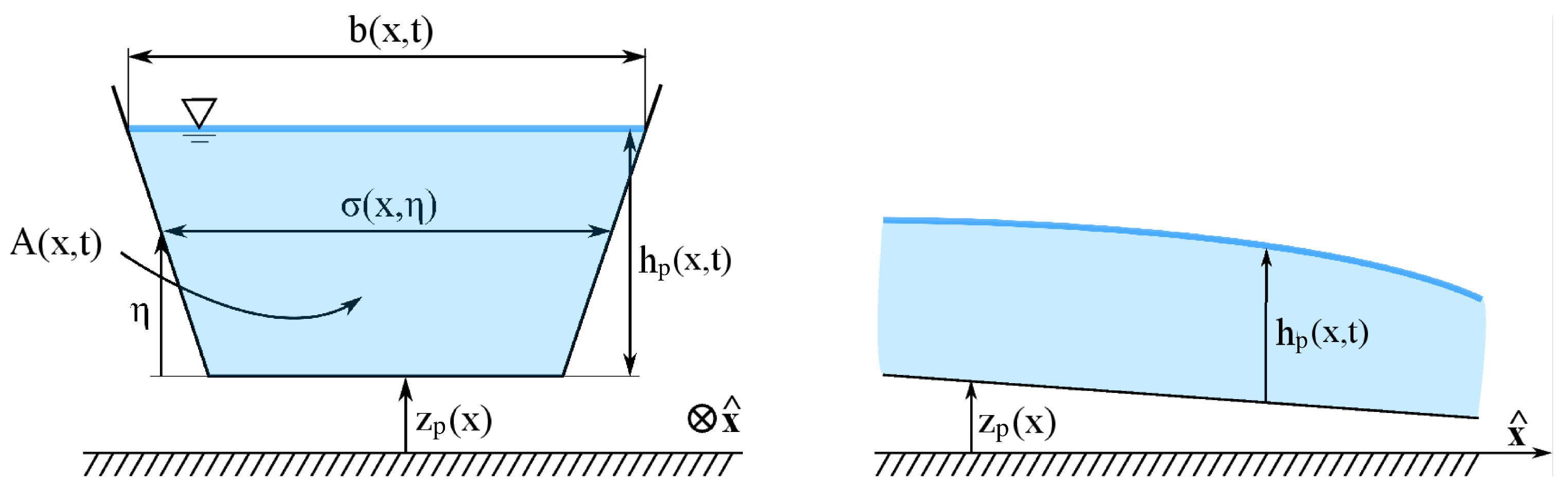
where $R=A/P$, P being the wetted perimeter. The coordinate system used for the formulation is shown in Figure 1. It is useful to rewrite the equation system in a vectorial form:

$$\frac{\partial \mathbf{U}}{\partial t}+\frac{\partial \mathbf{F}}{\partial x}=\mathbf{R},$$

(20)

where

$$\mathbf{U}={\left(A,Q\right)}^T,\mathbf{F}={\left(Q,\frac{Q^2}{A}+g{I}_1\right)}^T,\mathbf{R}={\left(0,g{I}_2+gA\left(S_0^{1D}-S_f^{1D}\right)\right)}^T$$

(21)

In cases in which $\mathbf{F}=\mathbf{F}\left(\mathbf{U}\right)$, when $I_2=0$, it is possible to rewrite the conservative system by means of the Jacobian matrix of the system:

$$\frac{\partial \mathbf{U}}{\partial t}+\mathbf{J}\frac{\partial \mathbf{U}}{\partial x}=\mathbf{R},\mathbf{J}=\frac{\partial \mathbf{F}}{\partial \mathbf{U}}=\left(\begin{array}{cc}0& 1\\ c^2-u^2& 2u\end{array}\right),$$

(22)

where c is the wave speed, defined as follows:

$$c=\sqrt{g\frac{\partial I_1}{\partial A}}.$$

(23)

The system matrix can be made diagonal by means of its set of real eigenvalues and eigenvectors, which represent the speed of propagation of the information:

$${\lambda }^{1,2}=u\pm c,{\mathbf{e}}^{1,2}={\left(1,u\pm c\right)}^T.$$

(24)

It is very common to characterize the flow type by means of the Froude number, $Fr=u/c$ (analogous to the Mach number in gases). This allows the classification of the flux into three main regimes: subcritical $Fr<1$, supercritical $Fr>1$, and critical $Fr=1$.

2.5. Preissmann Slot

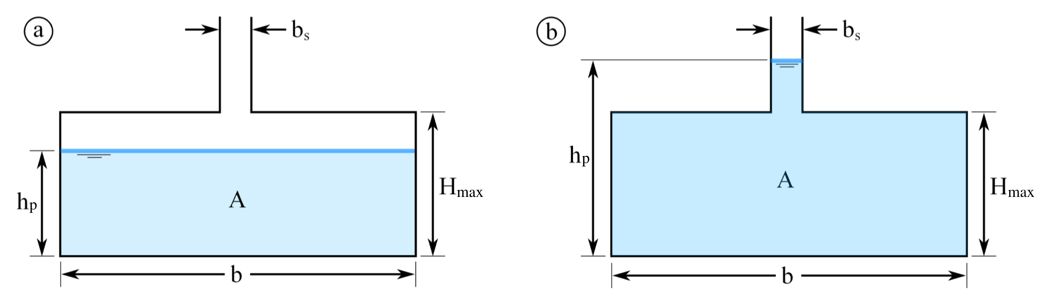
The Preissmann slot approach assumes that the top of the pipe or closed channel is connected to a hypothetical narrow slot, open to the atmosphere, so the shallow water equations can be applied with inclusion of this slot (see Figure 2). The slot width is ideally chosen to equal the speed of gravity waves in the slot to the water hammer wavespeed, so that the water level in the slot is equal to the pressure head level. The water hammer flow comes from the capacity of the pipe system to change the area and fluid density, so forcing the equivalence between both models requires the slot to store as much fluid as the pipe would by means of a change in area and fluid density. The pressure term and the wavespeed, assuming reactangular cross section, for $A\le b{H}_{max}$ are

$$h_p=\frac{A}{b}$$

(25)

$$I_1=\frac{A^2}{2b}$$

(26)

$$c=\sqrt{g\frac{\partial I_1}{\partial A}}=\sqrt{g\frac{A}{b}}$$

(27)

and for $A>b{H}_{max}$,

$$h_p=H_{max}+\frac{A-b{H}_{max}}{b_s}$$

(28)

$$I_1=b{H}_{max}\left(\frac{A-b{H}_{max}}{b_s}+\frac{H_{max}}{2}\right)+\frac{{(A-b{H}_{max})}^2}{2b_s}$$

(29)

$$c=\sqrt{g\frac{\partial I_1}{\partial A}}=\sqrt{g\frac{A}{b_s}}.$$

(30)

The ideal choice for the slot width results in

$$c_{WH}=c\Rightarrow b_s=g\frac{A_f}{c_{WH}^2},$$

(31)

in which $A_f$ is the full pipe cross-section.

2.6. Exchange between Submodels

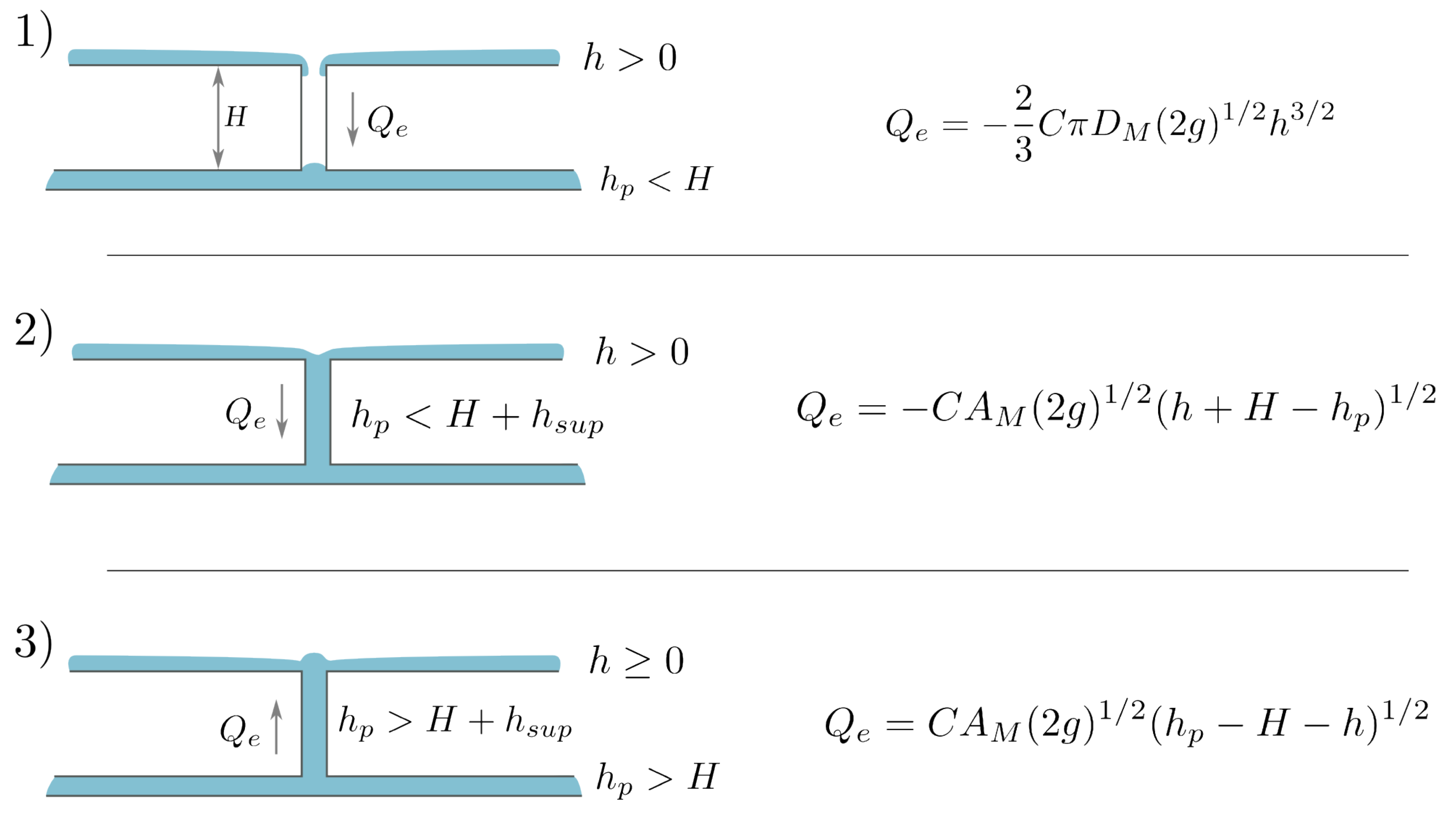
Several situations regarding the flow exchange between the surface flow and the sewer system can take place. Figure 3 displays all the possible scenarios: (1) inflow into non-pressurized sewer; (2) inflow into pressurized sewer; (3) outflow over a floodplain (wet or dry). For every time step, an internal algorithm compares the values of the surface water depth (h), pressure head in the pipe ($h_p$), and the distance between the bed of the flume and the inverted level of the sewer ($H=z+(z_p+H_{max})$) in order to adequately estimate the exchange discharge in terms of the diameter of the manhole ($D_M$), the area of the manhole ($A_M$), and a coefficient (C) which account for the energy losses at the manhole. The particular form used to formulate the exchange discharge ($Q_e$) closely follows the formulation suggested in reference [35].

2.7. Time Step Synchronization

The 1D system is solved by means of a finite volume scheme using an explicit time discretization [36], and therefore, it requires a control on the time step in order to avoid numerical instabilities. Hence, the Courant–Friedrichs–Lewy (CFL) condition is applied as

$$\Delta t_{1D}=\mathrm{CFL}\min \left(\frac{\Delta x_i}{|\widetilde{{\lambda }_i}|}\right)$$

(32)

where ${\lambda }_i$ are the eigenvalues of the 1D Jacobian, and the maximum CFL number is 1.

The coupled model can be built by combining the explicit drainage model with either the explicit 2D surface model (COUPLEDEX) or with the implicit 2D surface model (COUPLEDIMP). As the computation progresses from the initial condition to the future times using a global time step, the fully explicit combination requires the most restrictive time step to be used, so that

$$\Delta t=\min (\Delta t_{1D},\Delta t_{2D}).$$

(33)

When the COUPLEDIMP approach is used, the global $\Delta t$ is given by $\Delta t_{1D}$, as the 2D surface model is not restricted by stability limits.

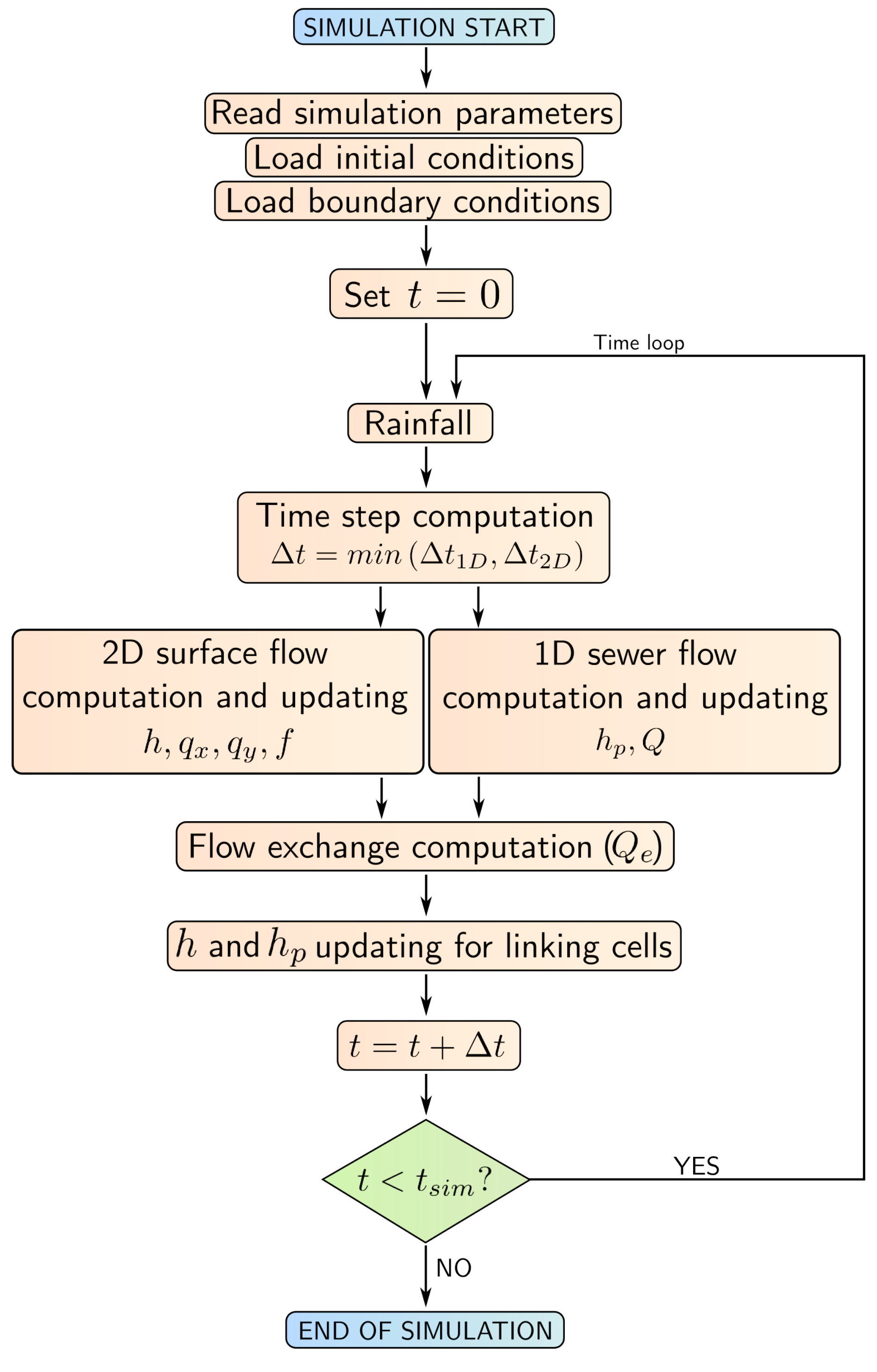
Figure 4 shows a schematic flowchart of the different model components.

3. Numerical Cases

3.1. Single Sewer/Surface Flow Exchange

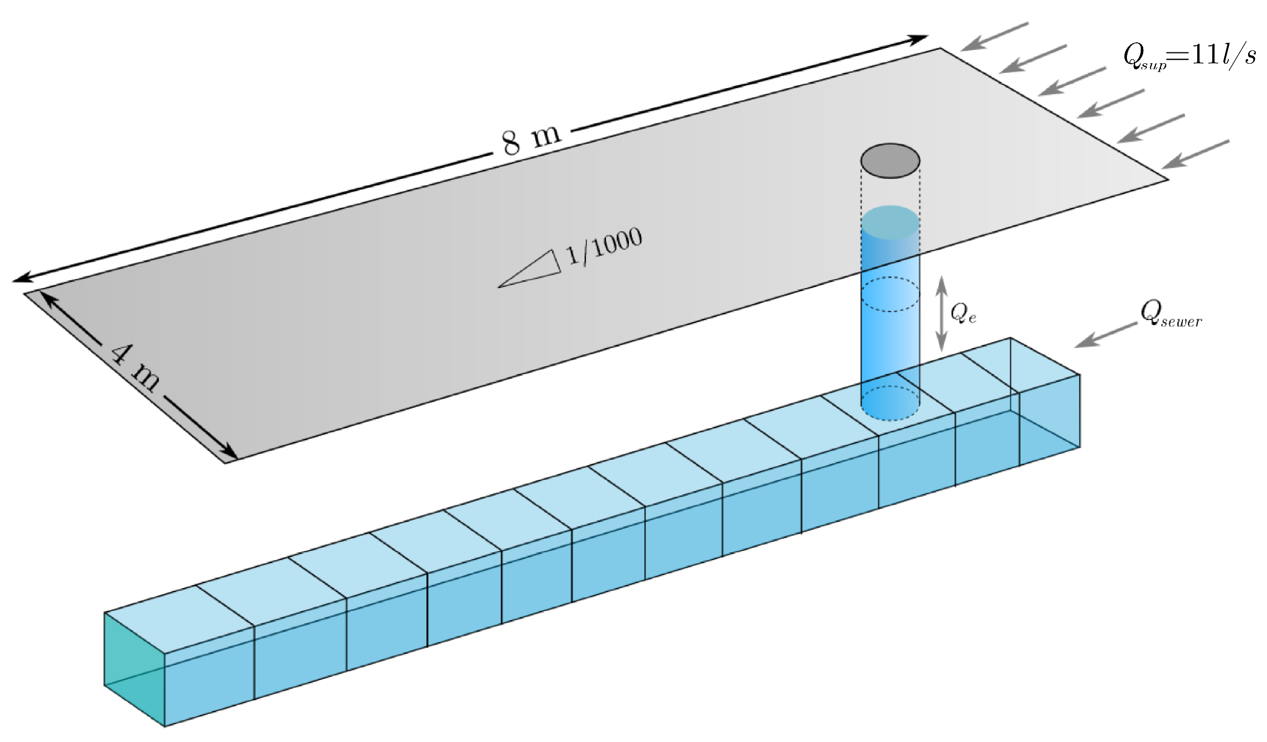
This test case was originally presented in reference [35] where a full range of sewer-to-surface and surface-to-sewer flow conditions at the exchange zone were experimentally analysed and hence, a complete set of observed data was provided. The experimental facility consists of a physical model of a sewer pipe with no slope connected via a manhole to a shallow flow flume (Figure 5). The sewer pipe has an internal width of $b=75$ mm. The flume bed has a slope of $S_0^{1D}=0.001$ and is aligned with the top of the manhole and is 4 m wide and 8 m long. The bed of the flume is $H=0.478$ m above the invert level of the pipe. All the facility components (pipe and flume) are constructed from PVC, so the Manning’s roughness coefficient is set to $n_{1D}=0.009$. This facility allows shallow flow over the surface which interacts with the sewer flow via the manhole. The boundary condition consists of a surface inlet discharge ($Q_{sup}=11$ L/s) and a sewer inlet discharge ($Q_{sewer}$), which varies depending on the case. The domain is assumed to be dry under initial conditions.

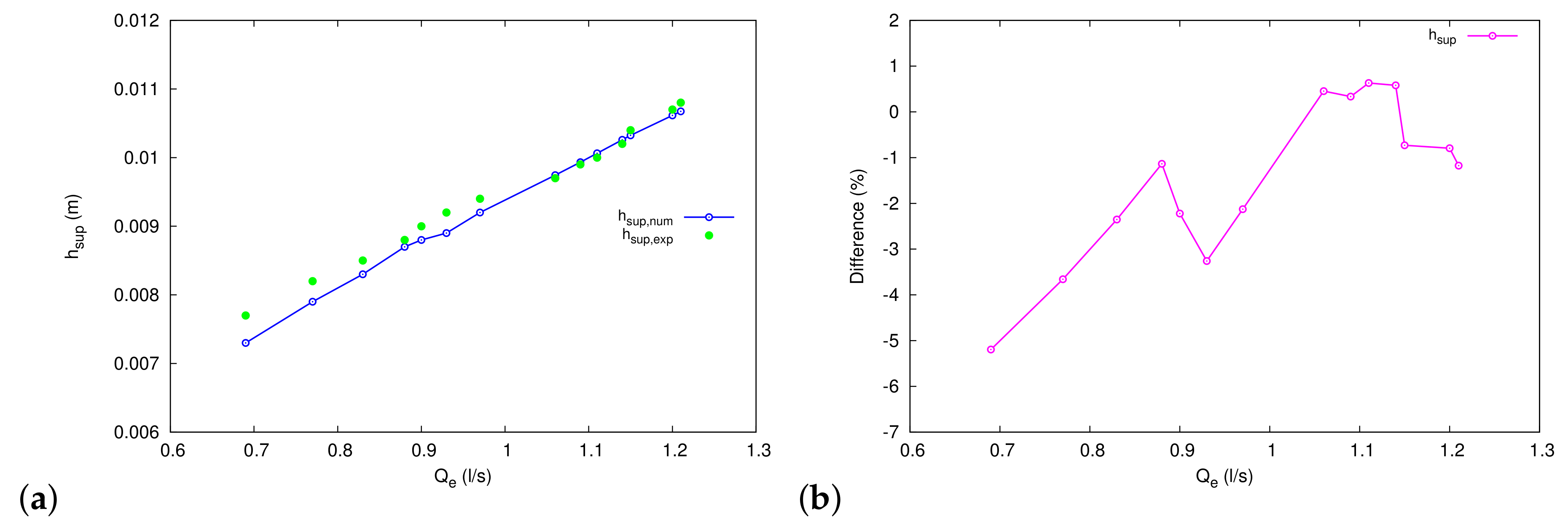
Two different cases were considered in this work. They cover all of the possible scenarios depicted in Figure 3. Case 1 was configured by setting zero discharge at the inlet of the sewer, leading to an inflow from the surface to the sewer throughout the case duration. Figure 6a shows the comparison between the numerical and experimental surface water depths for several values of $Q_e$, showing a very good overall agreement. The chosen values of $Q_e$ correspond to those in which data were available [35]. The relative differences between numerical and experimental data are plotted in Figure 6b, where a maximum error of $5\%$ is observed. The experimental data was measured 460 mm before the the center of the manhole for the surface water depth and 350 mm for the pipe pressure head.

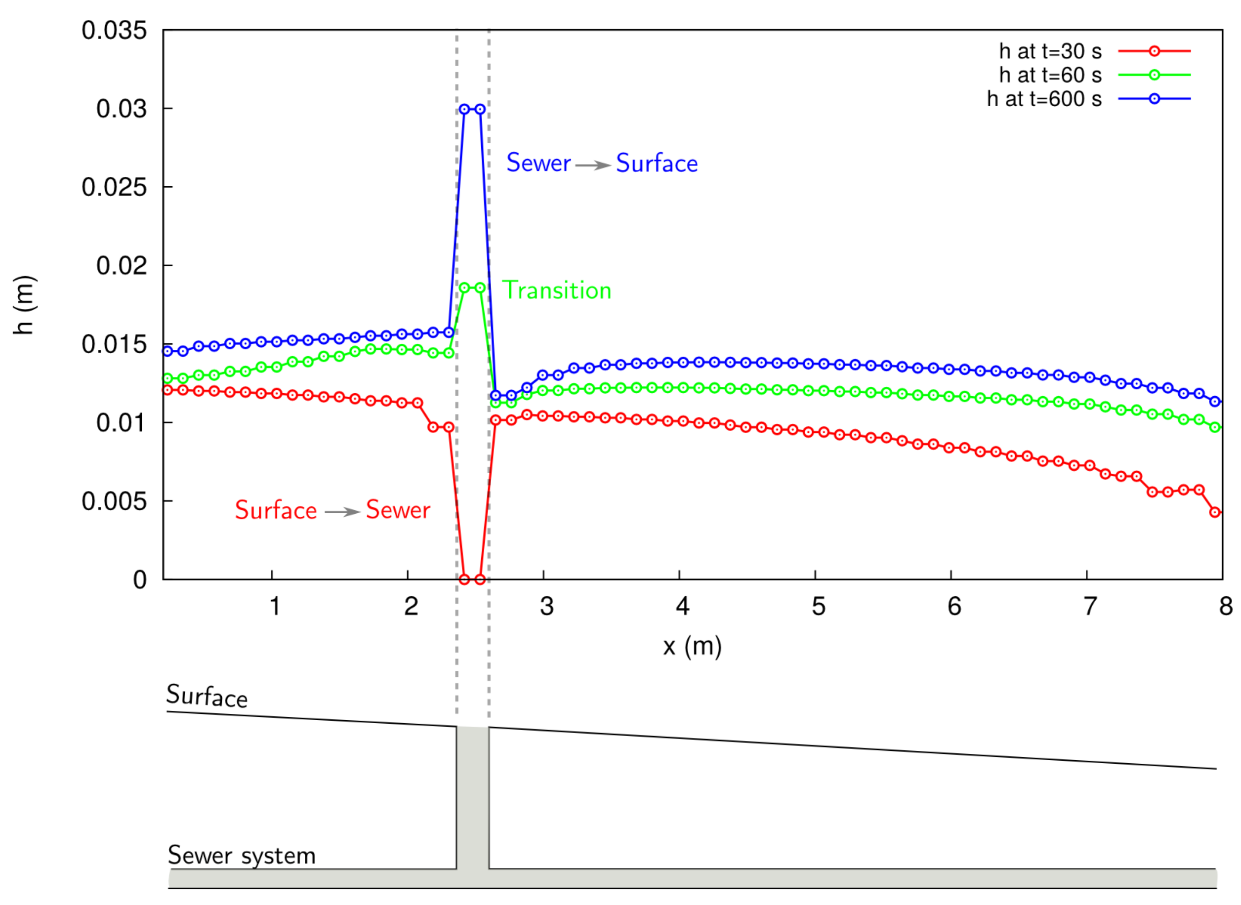
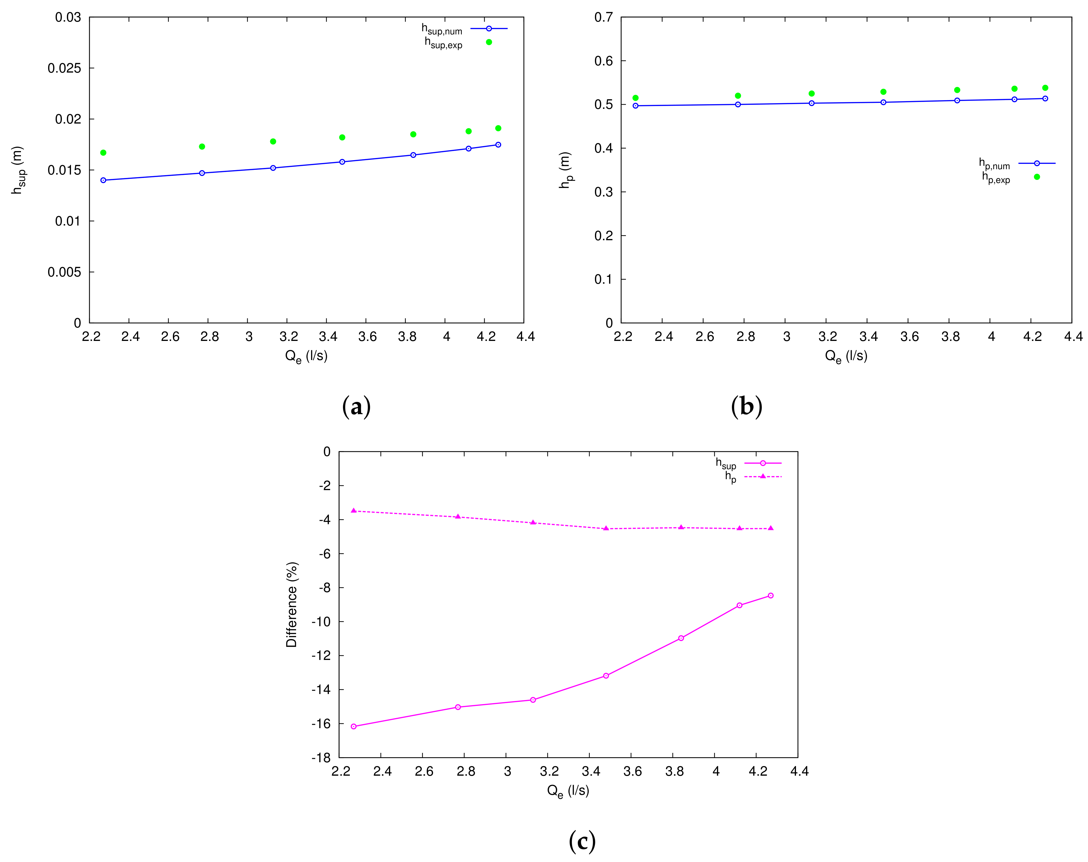
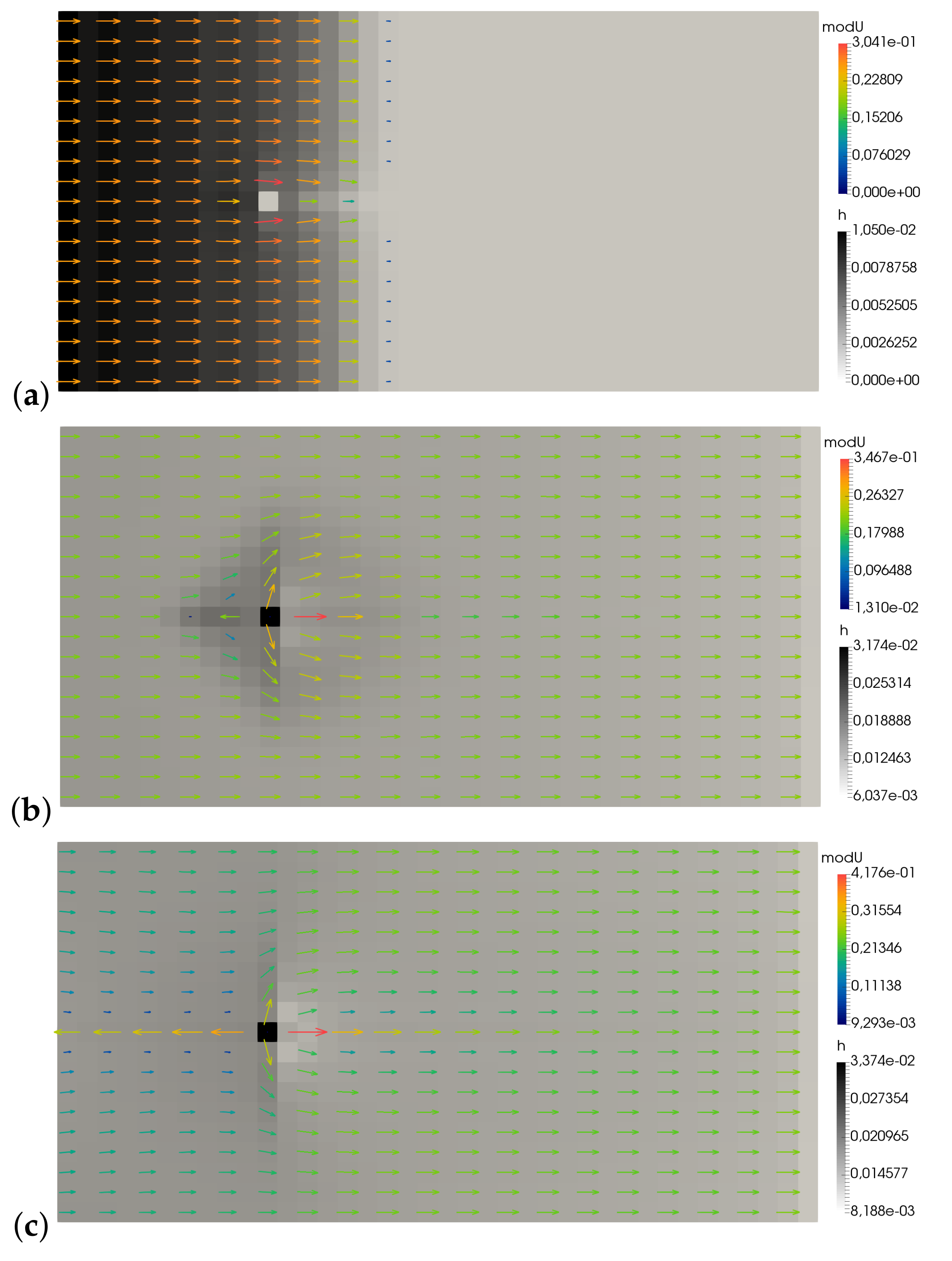
For Case 2, $Q_{sewer}=9.6$ L/s was set at the sewer inlet in order to ease the conduit pressurization. At the beginning of the simulation, water flows from the surface to the sewer (inflow) but, as the pipe pressure increases, the situation reverses (outflow), as shown in the profile view of the numerical results in Figure 7. At $t=30$ s, the surface to sewer situation occurs, leading to a depression in the surface water level at the manhole position (red line). The conduit is filled progressively and becomes pressurized in a transition situation denoted with a green line in Figure 7. When the pressure head in the sewer is enough, the exchange flow discharge changes sign and the water overloads the pipe and arises to the surface (blue line). Figure 8 shows the comparison between the numerical and experimental data for the surface water depth (a) and pressure head in the sewer (b). The relative differences for both magnitudes are shown in Figure 8c with a maximum of $15\%$ for the surface water depth and $5\%$ for the pressure head. A distributed visualization of the 2D numerical results at three different times is shown in Figure 9 with the water depth displayed in grayscale and the velocity vector field in color scale. The transition between inflow and outflow situations is clearly shown.

3.2. Application to a Case Study

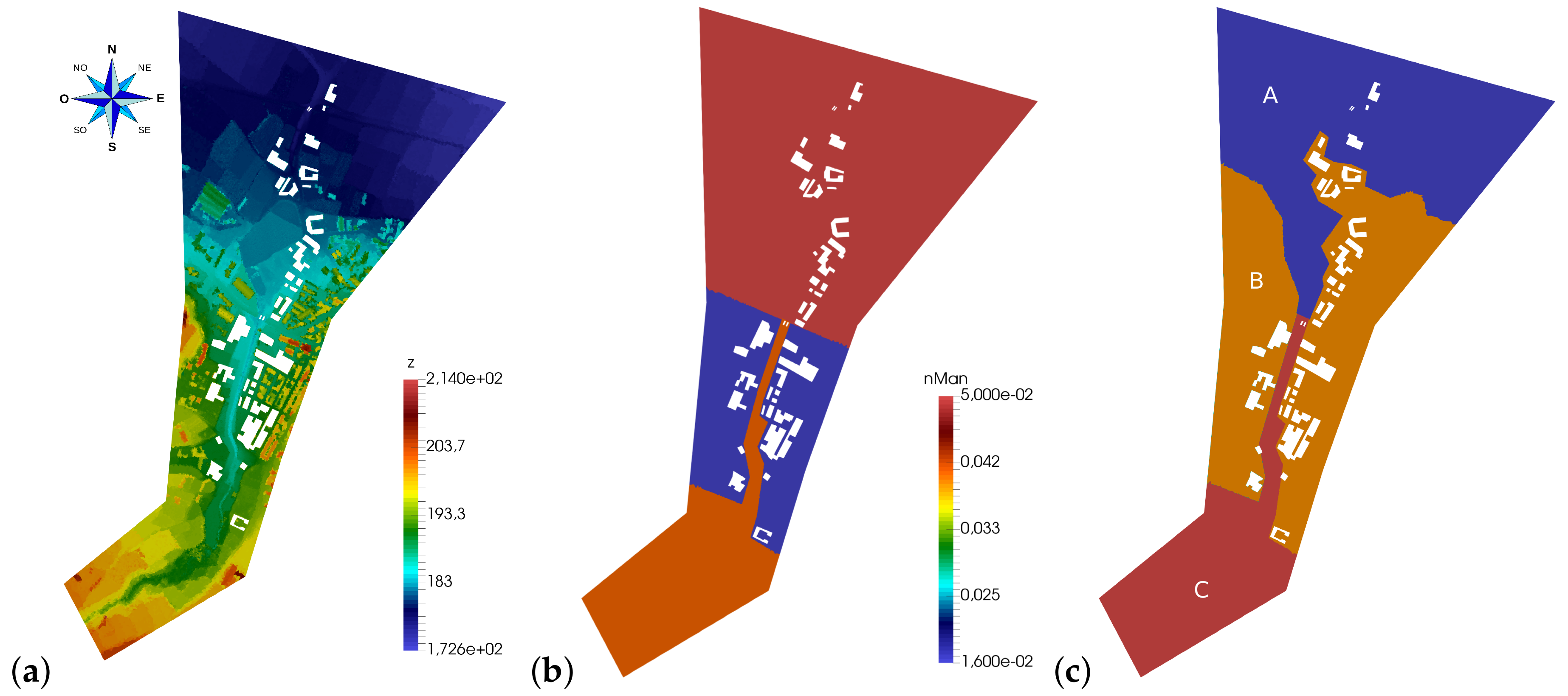
The Ginel river is a right bank tributary to the Ebro river in Spain. It is a small (77.3 km${}^2$) river basin, long and narrow in shape, with a length of 17.3 km and SW–NW oriented. The upstream and downstream bed levels are 328 m and 165 m, respectively (see Figure 10a), hence leading to an average longitudinal slope of $0.9\%$.

The case study focused on an approximately 600 m region of the urban reach of the river through the town of Fuentes de Ebro (Zaragoza, Spain). Figure 10b shows the spatial distribution of the Manning roughness coefficient used which ranged from $n=0.04$ s m${}^{-1/3}$ in the main channel, to $n=0.016$ s m${}^{-1/3}$ in the urban area and assumed $n=0.05$ s m${}^{-1/3}$ on the downstream area where there is more vegetation. The regions used for infiltration parameters can be seen in Figure 10c.

Table 1. Horton infiltration model parameters.

Zone	k (s${}^{-1}$)	${\mathit{f}}_0$ (m/s)	${\mathit{f}}_{\mathit{c}}$ (m/s)
A	$0.0001$	$1.9\times {10}^{-6}$	$1.0\times {10}^{-6}$
B	$0.0001$	$1.9\times {10}^{-8}$	$1.0\times {10}^{-8}$
C	$0.0001$	$1.9\times {10}^{-7}$	$1.0\times {10}^{-7}$

includes the Horton model parameters used.

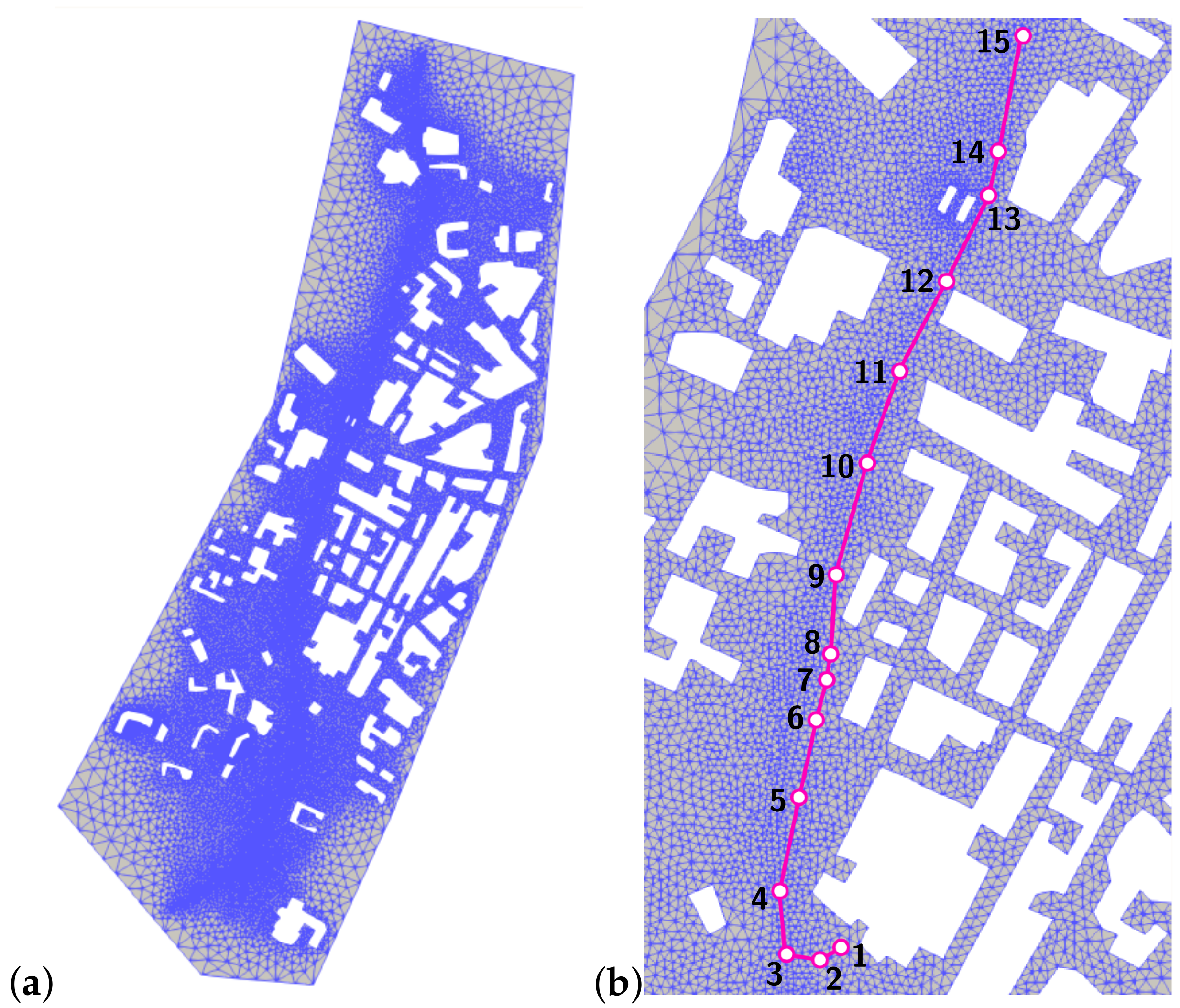
The 2D surface domain was discretized using an unstructured triangular flexible mesh of 29,600 cells. The mesh was locally refined near the main channel and in the area between the buildings. Bed elevations were obtained from a 2 m × 2 m Digital Terrain Model (DTM) completed with 842 in situ topographical data. Figure 11a shows the 2D surface computational mesh.

The drainage network geometry is shown in Figure 11b. It forms the main drainage conduit of the town and is located parallel to the main river channel. The 15 culvert connection positions are also shown in Figure 11b. The section of the conduit is considered to be 0.75 m × 0.75 m squared. Almost all of the network is made of concrete, so a Manning roughness coefficient of 0.03 s m${}^{1/3}$ was assumed all along the drainage system. A discretization with a cell size of $\Delta x=1$ m was set for all 1D domains, leading to a 500 cell mesh. As the initial condition, a constant water depth of 7 mm was assumed. A constant discharge of 10 L/s was set as the upstream boundary condition, whereas free flow was assumed downstream.

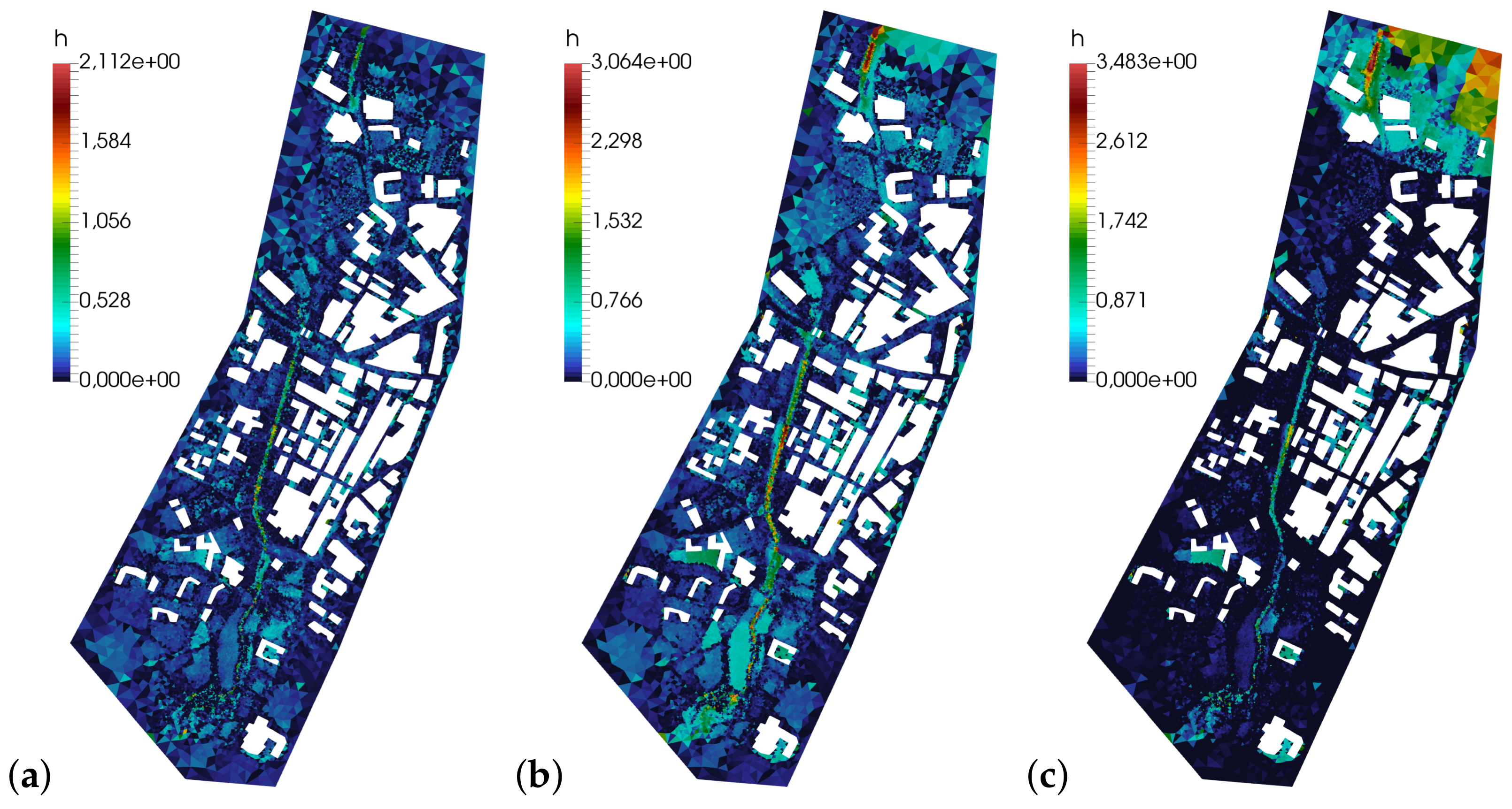
Two simulations with different initial conditions were performed. First, a heavy constant rainfall of 0.7 mm/s with a duration of 600 s was assumed over the entire domain, which was initially dry (Case 2.1). In the second test (Case 2.2), a surface water depth of 2 m was imposed upstream in order to simulate the peak level of an extraordinary flood situation. The purpose of both tests was to evaluate the sewer system’s capability to drain the excess surface water under these two assumptions. The use of a distributed surface flow model allowed us to calculate every hydraulic/hydrologic variable, such as the water depth (h), velocities ($u,v$) and infiltration rate (f), individually for each cell of the computational mesh. Hence, the available information is much larger that the results provided by a lumped simulation model.

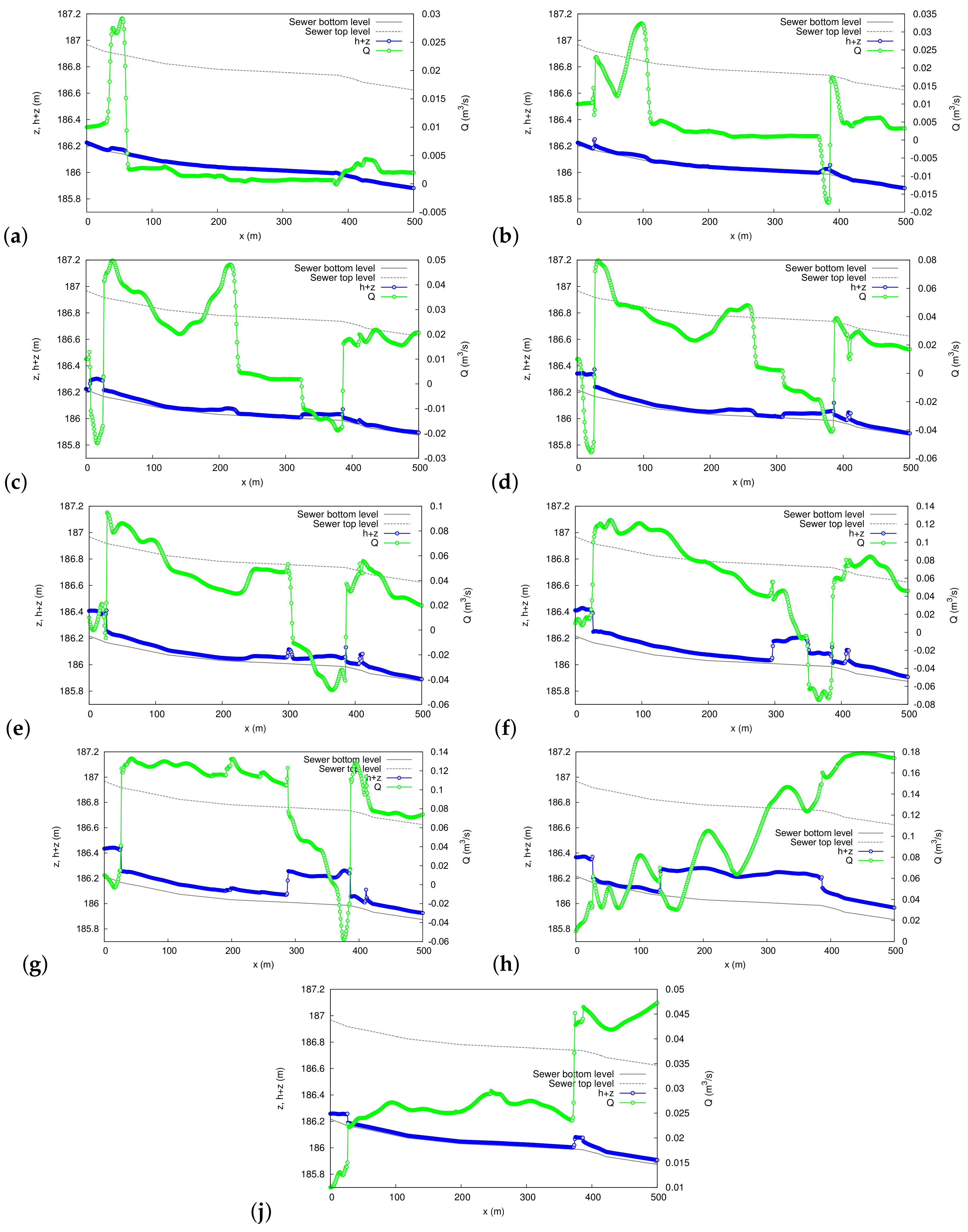
Figure 12 shows the simulated water surfaces at $t=150$ s (a), 300 s (b), and 3000 s (c) for Case 2.1. The huge intensity and short duration of the storm modelled generates large water depth values (up to 3 m) in the main channel of the river and at several punctual locations. Figure 13 shows the water level ($h_p+z$) within the drainage system and the instant discharge (Q) for nine instances of the simulation. The bottom and top levels of the sewer are also shown. The contribution from the surface flow through the culverts is clearly seen in the form of water level peaks where the surface-sewer connection is located (Figure 13). The drainage system was able to absorb the excess of surface water for the entire time of the simulation.

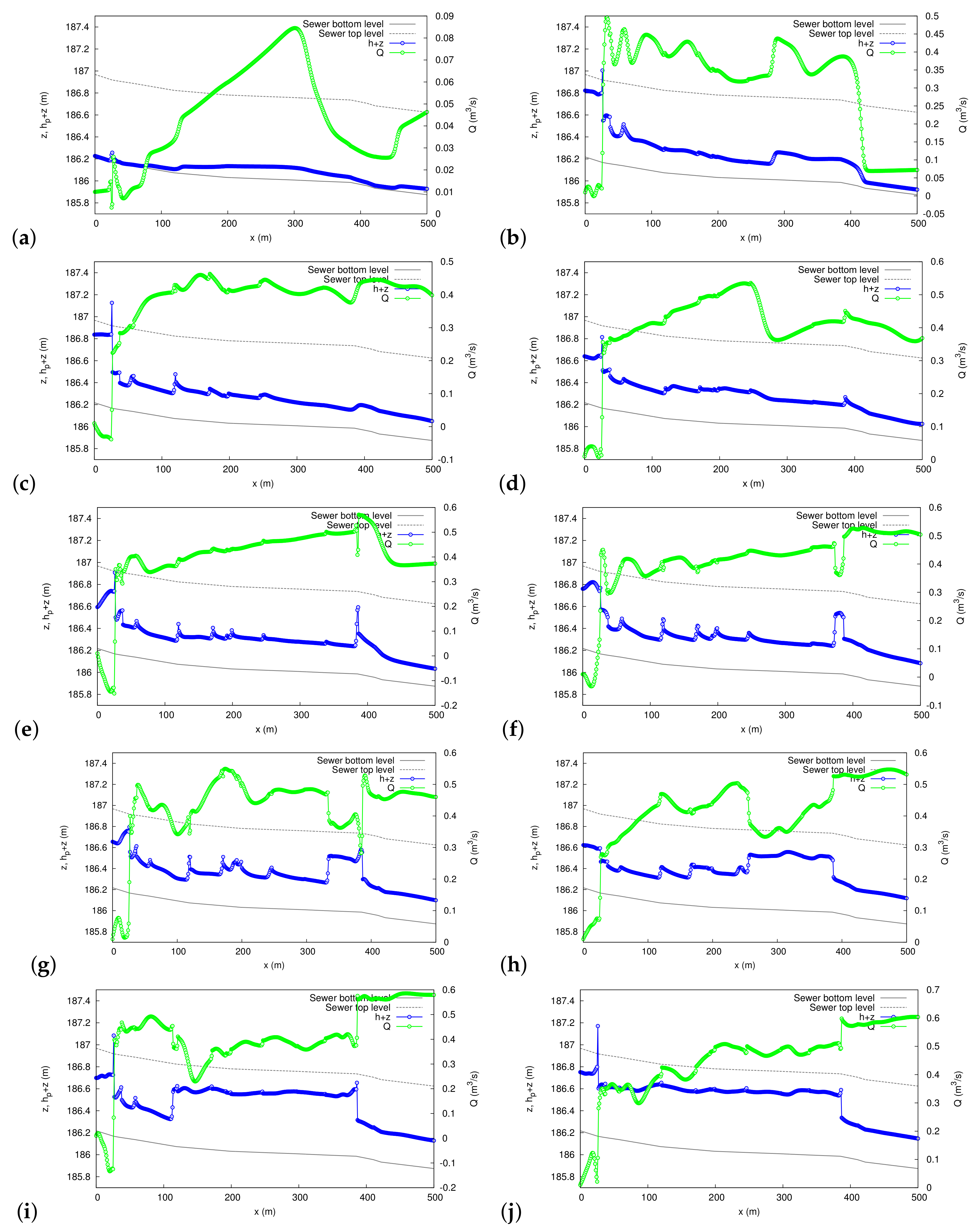
Figure 14 shows the surface water depth values at $t=60$ s, 150 s, 300 s, 750 s, 1000 s, and 2500 s for Case 2.2. The figures show the progression of the flood wave along the urban area, overflowing the main channel in some points, with water depth values of 5 m. Figure 15 shows the water level ($h_p+z$) within the drainage system and the instant discharge (Q) for 10 simulation times. As in Case 2.1, the surface water contributions are clearly seen along the sewer. In this case, the sewer was puntually pressurized, but the coupled model was able to deal with this kind of situation without any issues. As there is no actual data to validate the modeled results for this test, it is not possible to verify their credibility, but the examples are useful to demonstrate that the coupling of the models provides stable time evolution of all the the variables, including the exchange discharge.

4. Conclusions

The implementation of a finite volume upwind scheme to solve the 2D shallow water equations and the 1D shallow water equations as well as their coupling was presented in this work. The leading interest is the possibility to provide dynamic simulations of the interaction between free surface flow on the surface and drainage flow in urban systems.

The coupled model was validated in both smooth-transient and steady situations through a test case with laboratory measured data in several configurations for the inlet discharge. An overall good coincidence with experimental results was obtained with maximum differences of approximately $5\%$ for the water depth in the unpressurized case and $5\%$ and $15\%$ in the pressurized situation for the water depth values and the pressured head, respectively.

A real world application was shown in the last part of the work. An intense and short pulse of rainfall was simulated over the detailed topography of Fuentes de Ebro (Zaragoza, Spain) in which the main sewer conduit together with 15 manholes was also modeled. Several infiltration and roughness regions were considered mainly in reegard to their soil characteristics. A locally-refined triangular mesh allowed a precise discretization of the surface domain with the optimal number of cells. The use of a complete 2D dynamic surface distributed model allowed access to detailed information concerning the spatial distributions and temporal evolution of water depth, velocity, infiltration rate, or any other hydraulic/hydrologic variable. Under two different assumptions for the initial conditions (heavy rainfall and flood event), both surface and sewer flow models predicted the instant evolution of the water depth in both domains (surface and sewer). This work shows that it is possible to adapt 2D surface flow models to drainage networks which can become locally pressurized.

References

- Vreugdenhil, C. Numerical Methods for Shallow Water Flow; Kluwer Academic Publishers: Dordrecht, The Netherlands, 1994. [Google Scholar]
- Murillo, J.; García-Navarro, P. Weak solutions for partial differential equations with source terms: Application to the shallow water equations. J. Comput. Phys. 2010, 229, 4327–4368. [Google Scholar] [CrossRef]
- Burguete, J.; García-Navarro, P. Efficient construction of high-resolution TVD conservative schemes for equation with source terms: Application to shallow water flows. Int. J. Numer. Methods Fluids 2001, 37, 209–248. [Google Scholar] [CrossRef]
- Brufau, P.; Vázquez-Cendón, M.E.; García-Navarro, P. A numerical model for the flooding and drying of irregular domains. Int. J. Numer. Methods Fluids 2002, 39, 247–275. [Google Scholar] [CrossRef]
- Brufau, P.; García-Navarro, P.; Vázquez-Cendón, M.E. Zero mass error using unsteady wetting-drying conditions in shallow flows over dry irregular topography. Int. J. Numer. Methods Fluids 2004, 45, 1047–1082. [Google Scholar] [CrossRef]
- Liang, Q.; Marche, F. Numerical resolution of well-balanced shallow water equations with complex source terms. Adv. Water Res. 2009, 32, 873–884. [Google Scholar] [CrossRef]
- Ponce, V. Diffusion Wave Modeling of Catchment Dynamics. J. Hydraul. Eng. 1986, 112, 716–727. [Google Scholar] [CrossRef]
- Cea, L.; Garrido, M.; Puertas, J. Experimental validation of two-dimensional depth-averaged models for forecasting rainfall-runoff from precipitation data in urban areas. J. Hydrol. 2010, 382, 88–102. [Google Scholar] [CrossRef]
- Fernández-Pato, J.; García-Navarro, P. 2D Zero-Inertia Model for Solution of Overland Flow Problems in Flexible Meshes. J. Hydrol. Eng. 2016, 21, 04016038. [Google Scholar] [CrossRef]
- León, A.S.; Ghidaoui, M.S.; Schmidt, A.R.; García, M.H. Application of Godunov-type schemes to transient mixed flows. J. Hydraul. Res. 2009, 47, 147–156. [Google Scholar] [CrossRef]
- García-Navarro, P.; Vázquez-Cendón, M. On numerical treatment of the source terms in the shallow water equations. Comput. Fluids 2000, 29, 951–979. [Google Scholar] [CrossRef]
- Kerger, F.; Archambeau, P.; Erpicum, S.; Dewals, B.J.; Pirotton, M. An exact Riemann solver and a Godunov scheme for simulating highly transient mixed flows. J. Comput. Appl. Math. 2010, 235, 2030–2040. [Google Scholar] [CrossRef]
- Trajkovic, B.; Ivetic, M.; Calomino, F.; D’Ippolito, A. Investigation of transition from free surface to pressurized flow in a circular pipe. Water Sci. Technol. 1999, 39, 105–112. [Google Scholar] [CrossRef]
- Burguete, J.; García-Navarro, P. Implicit schemes with large time step for non-linear equations: Application to river flow hydraulics. Int. J. Numer. Methods Fluids 2004, 46, 607–636. [Google Scholar] [CrossRef]
- García-Navarro, P.; Alcrudo, F.; Priestley, A. An implicit method for water flow modelling in channels and pipes. J. Hydraul. Res. 1994, 32, 721–742. [Google Scholar] [CrossRef]
- Casoulli, V. Semi-implicit finite difference methods for the two-dimensional shallow water equations. J. Comput. Phys. 1990, 86, 56–74. [Google Scholar] [CrossRef]
- Kärnä, T.; de Brye, B.; Gourgue, O.; Lambrechts, J.; Comblen, R.; Legat, V.; Deleersnijder, E. A fully implicit wetting–drying method for DG-FEM shallow water models, with an application to the Scheldt Estuary. Comput. Methods Appl. Mech. Eng. 2011, 200, 509–524. [Google Scholar] [CrossRef]
- Li, S.; Duffy, C.J. Fully-Coupled Modeling of Shallow Water Flow and Pollutant Transport on Unstructured Grids. Procedia Environ. Sci. 2012, 13, 2098–2121. [Google Scholar] [CrossRef]
- Bagheri, J.; Das, S. Modeling of Shallow-Water Equations by Using Implicit Higher-Order Compact Scheme with Application to Dam-Break Problem. J. Appl. Comput. Math. 2013, 2, 1000132. [Google Scholar]
- Tavelli, M.; Dumbser, C. A high order semi-implicit discontinuous Galerkin method for the two dimensional shallow water equations on staggered unstructured meshes. Appl. Math. Comput. 2014, 234, 623–644. [Google Scholar] [CrossRef]
- Kesserwani, G.; Liang, Q. RKDG2 shallow-water solver on non-uniform grids with local time steps: Application to 1D and 2D hydrodynamics. Appl. Math. Model. 2015, 39, 1317–1340. [Google Scholar] [CrossRef] [Green Version]
- Chen, A.; Hsu, M.; Chen, T.; Chang, T. An integrated inundation model for highly developed urban areas. Water Sci. Technol. 2005, 51, 221–229. [Google Scholar] [CrossRef] [PubMed]
- Djordjevic, S.; Prodanovic, D.; Ivetic, M.; Savic, D. SIPSON simulation of interaction between pipe flow and surface overland flow in networks. Water Sci. Technol. 2005, 52, 275–283. [Google Scholar] [CrossRef] [PubMed]
- Fraga, I.; Cea, L.; Puertas, J. Validation of a 1D-2D dual drainage model under unsteady part-full and surcharged sewer conditions. Urban Water J. 2017, 14, 74–84. [Google Scholar] [CrossRef]
- Fraga, I.; Cea, L.; Puertas, J.; Suárez, J.; Jiménez, V.; Jácome, A. Global sensitivity and GLUE-based uncertainty analysis of a 2D-1D dual urban drainage model. J. Hydrol. Eng. 2016, 21, 04016004. [Google Scholar] [CrossRef]
- Hsu, M.; Chen, S.; Chang, T. Inundation simulation for urban drainage basin with storm sewer system. J. Hydrol. 2000, 234, 21–37. [Google Scholar] [CrossRef] [Green Version]
- Leandro, J.; Chen, A.; Djordjevic, S.; Savic, D. Comparison of 1D/1D and 1D/2D coupled (sewer/surface) hydraulic models for urban flood simulation. J. Hydraul. Eng. 2009, 135, 495–504. [Google Scholar] [CrossRef]
- Leandro, J.; Djordjevic, S.; Chen, A.; Savic, D.; Stanic, M. Calibration of a 1D/1D urban flood model using 1D/2D model results in the absence of field data. Water Sci. Technol. 2011, 64, 1016–1024. [Google Scholar] [CrossRef] [PubMed]
- Seyoum, S.; Vojinovic, Z.; Price, R.; Weesakul, S. Coupled 1D and non inertia 2D flood inundation model for simulation of urban flooding. J. Hydraul. Eng. 2011, 138, 23–34. [Google Scholar] [CrossRef]
- Horton, R. The role of infiltration in the hydrologic cycle. Trans. Am. Geophys. Union 1933, 14, 446–460. [Google Scholar] [CrossRef]
- Rawls, W.; Yates, P.; Asmussen, L. Calibration of Selected Infiltration Equation for the Georgia Coastal Plain; Report ARS-S-113; Agriculture Research Service: Washington, DC, USA, 1976. [Google Scholar]
- American Society of Civil Engineers (ASCE). Hydrology Handbook, 2nd ed.; American Society of Civil Engineers (ASCE): Reston, VA, USA, 1996. [Google Scholar]
- Fernández-Pato, J.; Morales-Hernández, M.; García-Navarro, P. Implicit finite volume simulation of 2D shallow water flows in flexible meshes. Comput. Methods Appl. Mech. Eng. 2018, 328, 1–25. [Google Scholar] [CrossRef]
- Murillo, J.; García-Navarro, P.; Burguete, J.; Brufau, R. The influence of source terms on stability, accuracy and conservation in two-dimensional shallow flow simulation using triangular finite volumes. Int. J. Numer. Methods Fluids 2007, 54, 543–590. [Google Scholar] [CrossRef]
- Rubinato, M.; Martins, R.; Kesserwani, G.; Leandro, J.; Djordjevic, S.; Shucksmith, J. Experimental calibration and validation of sewer/surface flow exchange equations in steady and unsteady flow conditions. J. Hydrol. 2017, 552, 421–432. [Google Scholar] [CrossRef]
- Fernández-Pato, J.; García-Navarro, P. Finite volume simulation of unsteady water pipe flow. Drinking Water Eng. Sci. 2014, 7, 83–92. [Google Scholar] [CrossRef]
Figure 1.
Coordinate system for shallow water equations.
Figure 2.
(a) Free surface pipe; (b) pressurized pipe.
Figure 3.
Possible hydraulic scenarios in the coupled model.
Figure 4.
Model flowchart.
Figure 5.
Scheme of the laboratory case setup.
Figure 6.
Case 1.1. Comparison between numerical and experimental data (a) and relative differences (%) (b) for the surface water depth.
Figure 7.
Profile view of the numerical results corresponding to three different times. Note the sign change of the exchange flow.
Figure 8.
Case 1.2. Comparison between numerical and experimental data for the surface water depth (a) and pressure head (b). Relative differences (%) between numerical and experimental data for the surface water depth and pressure head (c).
Figure 9.
Distributed numerical results for the overland flow corresponding to the water depth in m (grayscale) and the velocity vectors in m/s (colored) at s (a), 37 s (b) and 50 s (c).
Figure 10.
Ginel river at Fuentes de Ebro: Elevation map in m (a), Manning roughness coefficients in s m (b) and infiltration regions (c).
Figure 11.
Flexible mesh used for the 2D model (a) and sewer network scheme together with link locations (b).
Figure 12.
Case 2.1. Water depth values (h) in m at s (a), 300 s (b) and 3000 s (c).
Figure 13.
Case 2.1. Network profile at s (a), 80 s (b), 150 s (c), 175 s (d), 200 s (e), 250 s (f), 300 s (g), 1000 s (h), and 2000 s (j).
Figure 14.
Case 2.2. Water depth values (h) in m at s (a), 150 s (b), 300 s (c), 750 s (d), 1000 s (e), and 2500 s (f).
Figure 15.
Case 2.2. Network profile at s (a), 350 s (b), 430 s (c), 500 s (d), 540 s (e), 565 s (f), 650 s (g), 800 s (h), 1000 s (i), and 2500 s (j).