A-DInSAR Performance for Updating Landslide Inventory in Mountain Areas: An Example from Lombardy Region (Italy)

Abstract

This work focuses on the capabilities and limitations of the Advanced Satellite SAR (Synthetic Aperture Radar) Interferometry (A-DInSAR) in wooded and mountainous regions, with the aim to get insights on the performances for studying slow-moving landslides. The considered critical issues are related to the SAR acquisition geometries (angle of incidence of the satellite line of sight, ascending and descending geometries) and to the physical and morphological features of the slopes (land use, aspect and slope angles), which influence the measuring points coverage. 26 areas in Lombardy Region (Italy), affected by known slope instability phenomena, have been analyzed through A-DInSAR technique, using COSMO-SkyMed images. The results allowed to outline general considerations about the effectiveness of A-DInSAR analysis of a single dataset (descending or ascending dataset), selected accordingly to the aspect of the slopes. Moreover, we aimed to quantitatively describe the capability to update the state of activity of several previously mapped landslides using satellite SAR Interferometry results. Although in a wooded and mountainous region, where the chances of retrieving radar targets for satellite SAR analysis are generally low, the A-DInSAR results have allowed to detect landslides’ reactivations or new landslides and to update the inventory for about 70% of the investigated areas.

1. Introduction

Identifying and mapping landslides is essential to reduce their social and economic impact, as landslides represent one of the major causes of damages to structures and infrastructure and of life losses [1,2,3,4], in many hilly and mountainous areas all over the world.

Landslide inventories and information about the state of activity are the main tools to plan strategically the security and the expansion of urbanized areas and to prevent the damages. Mapping and studying landslides at large scale is therefore crucial for land use planning, but it can represent a goal hard to achieve through traditional “on-site” methods, due to the extension of regional areas of interest and the difficult accessibility. In this regard, remote sensing methods provide an effective solution to this problem, thanks to the capability to analyze wide areas at a low cost. Among these techniques, satellite SAR (Synthetic Aperture Radar) Interferometry (InSAR) is one of the most used remote sensing technologies for landslides mapping and for assessing slope stability, without installing instrumentation [5,6,7,8,9,10,11,12,13,14,15,16,17,18,19,20,21].

Different types of landslide mapping can be performed, such as landslide inventory, which represents a picture of an area at a given moment [22], landslide typology and landslide state of activity maps which requires hypothesis also about the temporal evolution of the processes [23]. Traditional landslide mapping procedure is generally affected by uncertainties and sometimes subjective information related to the surveyor expertise.

The evaluation of the state of activity, the style of activity and the intensity of a landslide [24]; i.e., destructiveness of a landslide, in terms of kinetic energy, volume, movement velocity or total displacement, etc.) represent usually complex tasks, due to the lack of a single standardized procedure for the quantification of these parameter [25,26].

Satellite InSAR has proven to be a reliable methodology for detecting ground deformation with sub-centimetric accuracy, and currently it is exploited by using multi-images processing approaches: The so-called Advanced Differential Synthetic Aperture Radar Interferometry, A-DInSAR, as for example the Persistent Scatterers Interferometry (PSI) [27,28,29]. A-DInSAR analysis represents a valuable tool for the updating of landslide inventories, and several attempts to assess the state of activity by using PSI results have been performed in the last decade [9,30,31]. Furthermore, several methodologies that integrate field surveys and conventional thematic data (e.g., topographic, geological, land use maps, and optical images) with Persistent Scatterer Interferometry (PSI) analyses have been designed [5,7,9,18,31,32,33,34,35]. Such techniques can detect geomorphologic phenomena not emerging from conventional field surveys and allow to modify landslide boundaries and to assess the landslide velocity and, therefore, evaluate the state of activity. Moreover, one of the key features of A-DInSAR is the ability to provide quantitative results about past ground displacements, providing the possibility to perform historical analyses, thanks to the data archives collected by the space agencies.

The increasing number of space missions, characterized by high performances in terms of both spatial and temporal resolution, are allowing the spread of monitoring services that control the evolution in time of the instability phenomena of interest. For the above-mentioned reasons, nowadays, the amount and availability of multi-temporal images are experiencing a fast increase, and the free access data policy adopted for missions like Sentinel (by European Space Agency, ESA) allows to take advantage of A-DInSAR technique at low cost. The satellites of new generation, with short revisit times, can be used for continuous and systematic tracking of ground deformation phenomena. In this regard, an example of innovative continuous monitoring of landslides at regional scale by means PSI data has been provided by Raspini et al. [32], with the transition from static satellite analysis, based on the analysis of archive images, to dynamic monitoring of ground displacement.

Despite the effectiveness and the low cost of A-DInSAR technique for landslide mapping and monitoring, which have been demonstrated and consolidated over the last 20 years, this methodology is not a routine analysis yet and it is not exploited as a standard practice by government authorities in charge of land management.

One of the reasons could lie in the complexity of the A-DInSAR analysis, and in the presence of some limitations typical of this technique that need to be addressed, as the interaction between the SAR acquisition geometries (ascending or descending) and the physical and morphological features of the slopes. This critical issue can directly affect the results both qualitatively and quantitatively: The measuring points coverage (number of PSs) is indeed strictly correlated with the slope orientation, which can be favorably oriented or not with respect to the satellite’s Line of Sight (LOS).

Colombo et al. [36] presented a model to predict PSs density, discarding those areas affected by layover and shadow effects and considering the land use. Notti et al. [14,35], proposed a predictive model to improve the use of Persistent Scatterers (PSs) techniques in the landslides study, introducing the RC-index that allows to forecast the potential PSs distribution, calculating the effects due to topography and land use. Cascini et al. [7] discussed and implemented the approach of a priori DInSAR landslide visibility mapping.

In this regard, this work aims to highlight how the physical and geometrical characteristics of the study area can influence the A-DInSAR results through a several cases studies in Lombardy Region (Italy). We analyzed 26 Areas of Interest (AOIs) affected by slope instability phenomena, that were indicated by the regional authority for environmental protection (Lombardy Regional Agency for Environmental Protection) in the framework of a project involving an A-DInSAR study [37]. These different case studies provided the opportunity to compare the results for each AOI and relate them to the morphological characteristics of the AOIs, in order to draw general considerations.

Moreover, the A-DInSAR analysis has been used to verify and possibly update the state of activity of the known landslides. These latter have been mapped in the Italian Landslide Inventory IFFI produced by the Italian Institute for Environmental Protection and Research [38,39,40]. The IFFI inventory provides a large amount of data performed on a reference scale of 1:10,000, employing aerial photointerpretation, field surveys, and local databases, but it needs to be integrated, validated and updated in order to support effectively the risk mitigation strategies. The version of the catalogue that has been used, is the IFFI of 2007, which preceded the time period investigated through satellite data.

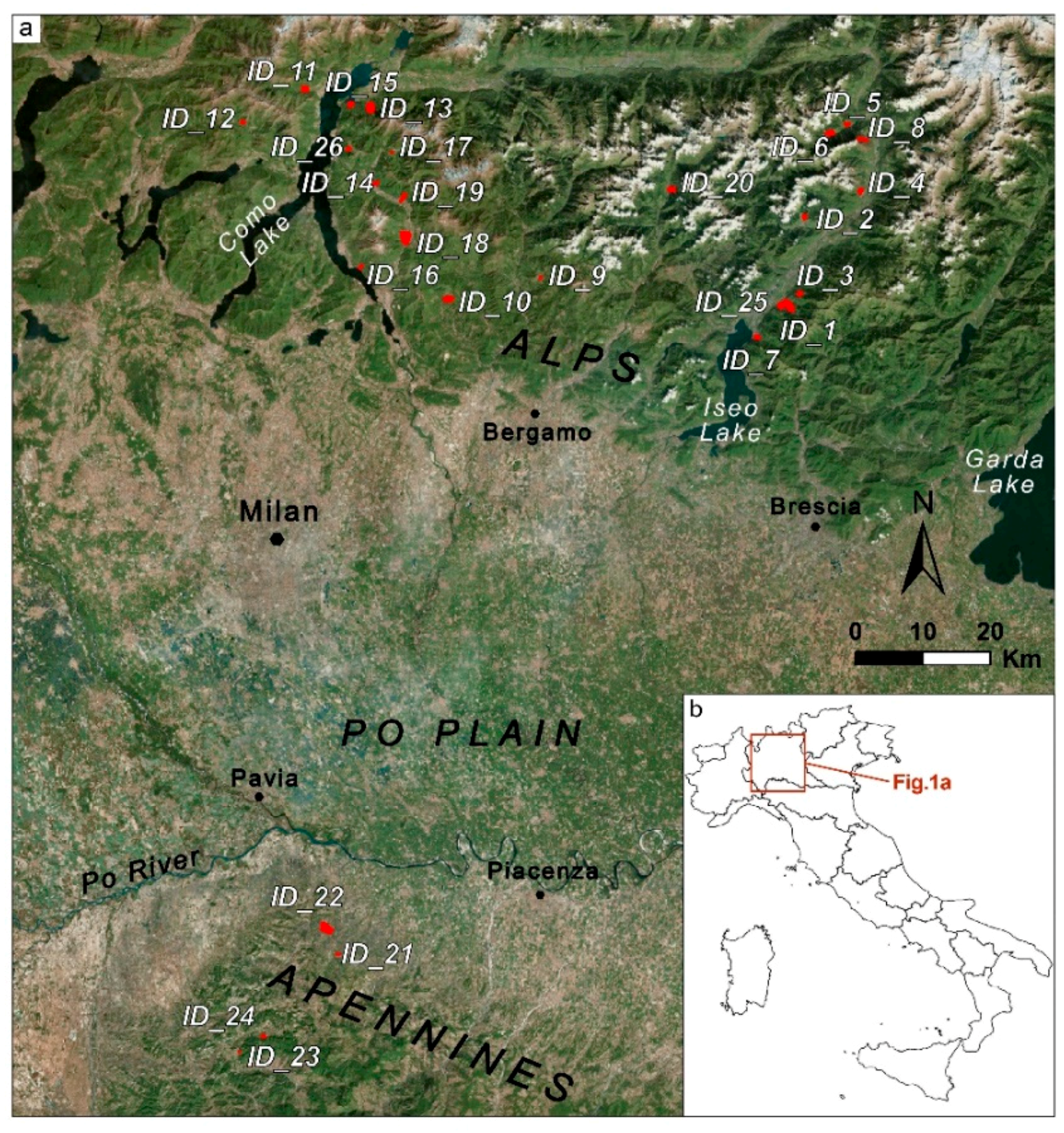
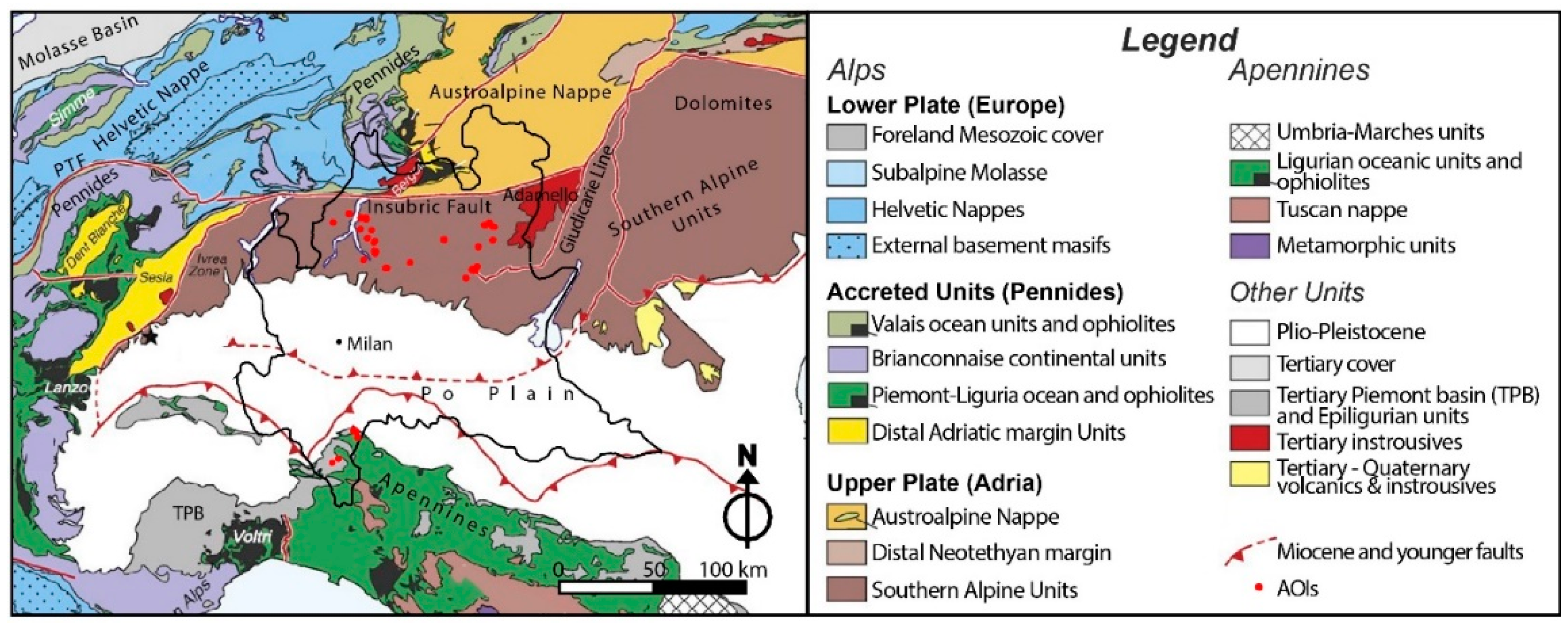
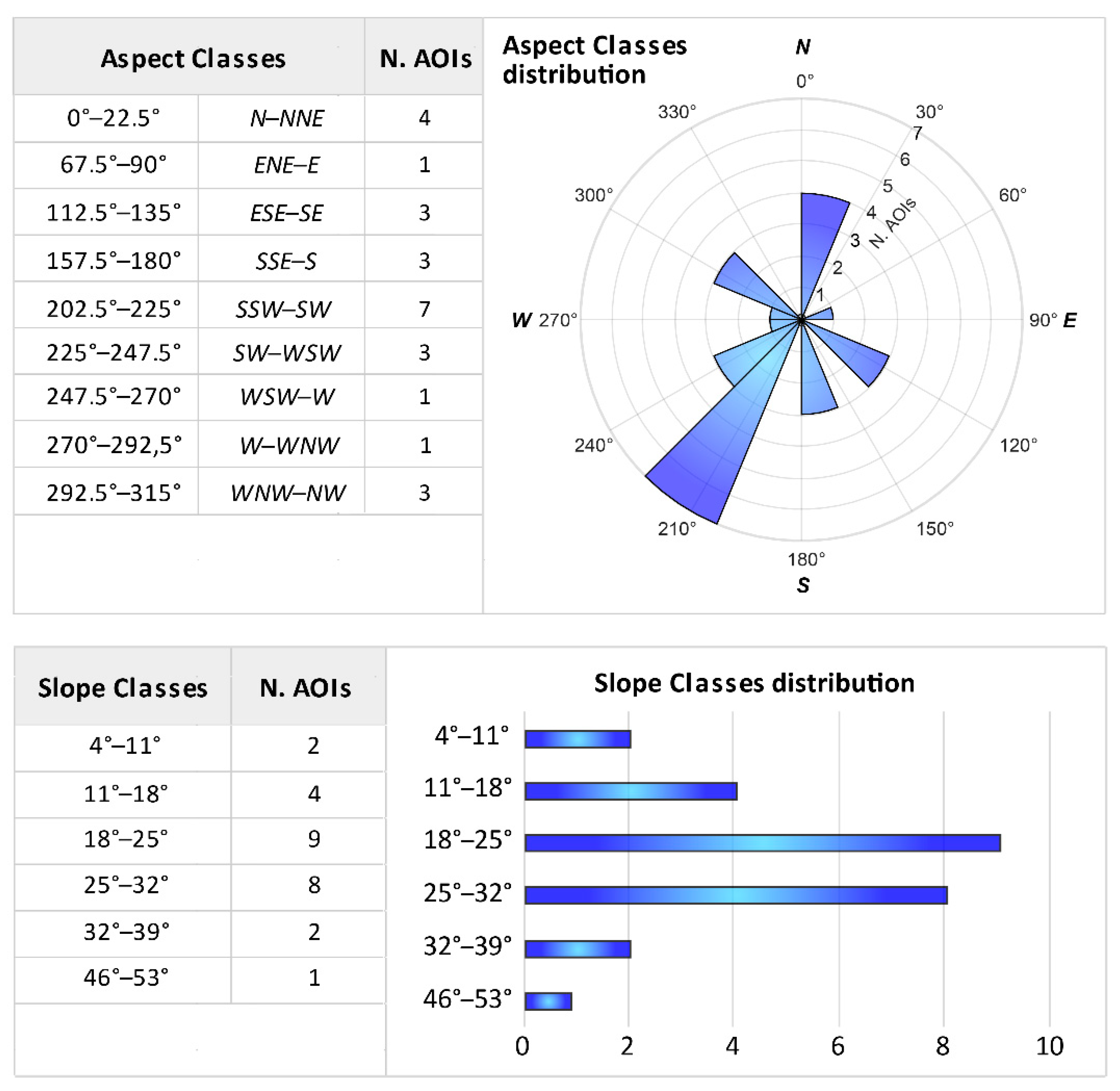
2. General Setting of the Study Areas

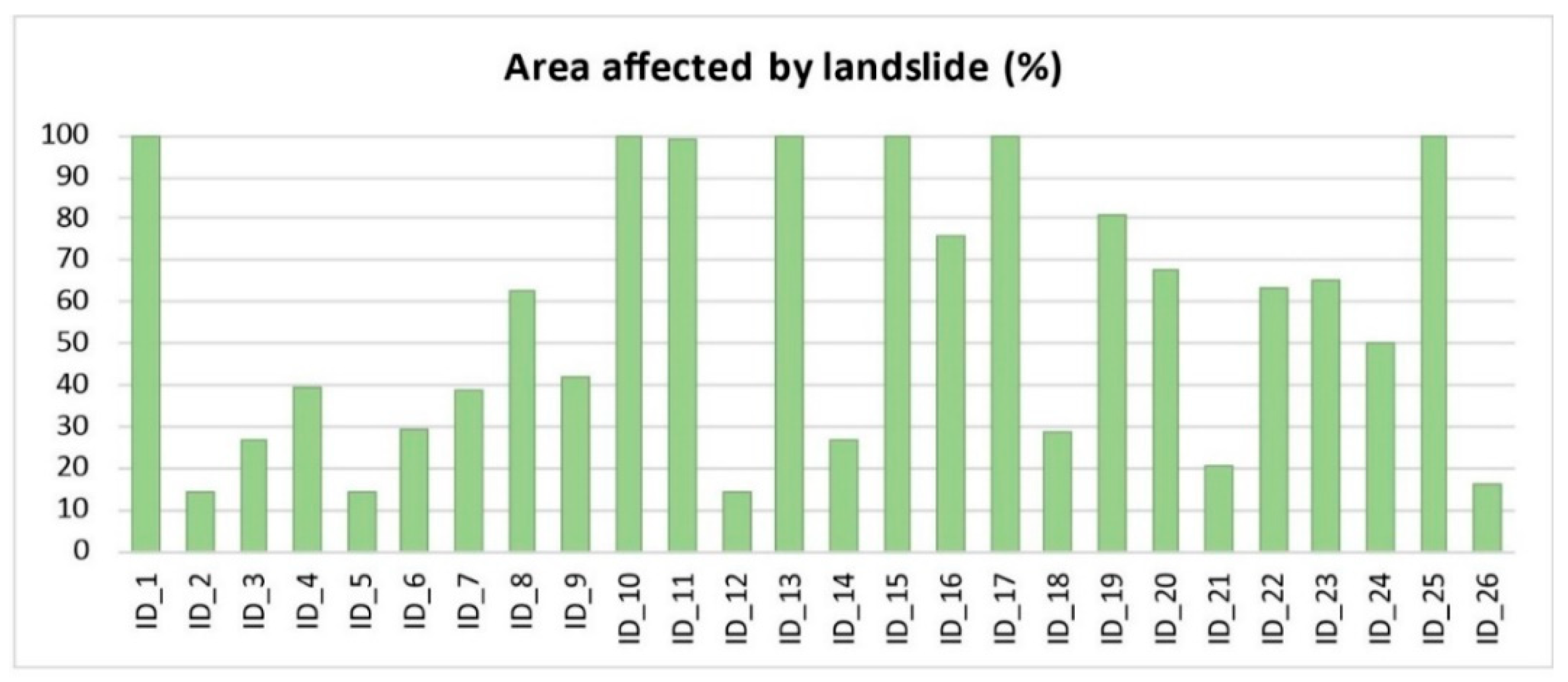
In this work, we studied 26 areas in Lombardy Region of Italy (AOIs; Figure 1) subjected to slope instability phenomena, and representing critical zones involving known landslides, mapped in the Italian Landslide Inventory (the so called IFFI inventory) [39]. The 26 AOIs have been indicated by the regional authority for environmental protection in accordance with the land management needs of the Lombardy Region.

22 AOIs occur in the Alpine chain and are located on the tectonic unit of Southern Alps (a), while 4 AOIs are located in the southernmost part of Lombardy the Oltrepò Pavese area (b), in the Apennine domain.

(a) The Southern Alps (Figure 2) of Lombardy Region consist of a minor, shallower (non-metamorphic) and younger (Neogene) thrust-and-fold belt displaced to south (Adria-verging), which developed within the Alpine hinterland of the Adriatic upper plate, far from the oceanic suture [41]. The Southern Alps are characterized by an Early Permian-Palaeogene succession of marine sediments since the Early Triassic [42], with a prevalence of carbonates (limestones, dolomites, and marls) and turbiditic sequences that outcrop in the Prealpine margin. The types of landslide that mainly occur in this sector are the translational slides [22] and debris flows. The area between the Pre-Alps and the Po Plain is characterized by widespread glacial, alluvial and fluvio-glacial deposits, which are affected generally by minor instability phenomena such as superficial sliding and collapses along the main escarpments [43].

(b) The Oltrepò Pavese, in Southern Lombardy, corresponds to the northwestern sector of the Apennines (Figure 2), characterized by a complex geological and structural setting [5]. The most widespread lithologies are clay-rich sedimentary formations of Cretaceous-Pliocene age [44]. The elevation ranges between 200 m and 1725 m a.s.l., and the slopes are in general slightly inclined (slope angles <20°); steeper slopes correspond to rock outcrops (limestone in the southern part and sandstone in the central part). The northern sector of the Oltrepò Pavese belongs to the Po River Plain, characterized by fluvial terraces and piedmont alluvial fans [5]. The geomorphological setting and the landscape evolution are essentially controlled by mass movements. Earth-slides and debris flows [22] occur frequently where the marine sediments and the marly-arenaceous deposits of the Appenine Units crops out [5].

In the most recent version of the IFFI database (Regione Lombardia, 2012) [40] the number of landslides mapped in the Lombardy region is 148.373, which correspond to anarea of over 4000 km². The greater density of the phenomena is found in the area of the Oltrepò Pavese and in the northernmost part of the region (Alta Valtellina and Valmalenco; Carelli, 2007, [43]). The frequency of landslides types in Lombardy are summarized in the histogram of Figure 3.

The most frequent type of landslide (about 37%) of Lombardy is earth or debris flow, involving superficial deposits, that are very common in the Alps and in the Pre-Alps slopes and torrent channels [40], and are often triggered by heavy rainfalls. The rock falls are also very widespread in the Lombard Alps, where steep and fractured cliffs occur, and represent about the 28% of the region’s landslides, while the earth and debris slumps and slides (both rotational and translational movements) represent the 20.6%. The areas subject to widespread shallow landslides are almost 6% of the total landslides in the region. Toppling and collapses (3.1% of occurring landslides) usually occur on rock slopes involving limited portions of territory [40].

As regards the state of activity of landslides in Lombardy Region, 61% of the phenomena assessed on a morphological basis, are active/reactivated/suspended. About the 34% of the landslides are quiescent, 2.5% are not determined (category: Undefined), and the remaining part (1.6%) is inactive. Only 0.2% of the surveyed landslides has been stabilized [40].

Some specific information about the AOIs has been extracted from the available thematic maps and databases, such as the geological map of Lombardy (scale 1:250,000), the land use map of the region (from CORINE Land Cover project), the SRTM (Shuttle Radar Terrain Model) with 30 × 30 m resolution, and the Italian Landslide Inventory IFFI [39,40]. This latter provides a standardize database with information about the landslide phenomena.

AOIs Description

The 26 AOIs studied in this work through satellite SAR interferometry, represent a very heterogeneous sample of zones with different settings: The AOIs have indeed different shape and size and differ in terms of land use and number of mapped landslides, thus providing a statistically sounding dataset. In fact, according to IFFI inventory, some AOIs include only few mapped landslides (or only one landslide), while others AOIs include several instability phenomena, with different state of activity. In Figure 4, three very different examples of AOIs are showed: ID_2 (Popoia) includes only one active landslide and a large part of the area is not affected by previously mapped instability phenomena; ID_5 (Paisco Loveno) includes a big landslide that covers almost the whole extent of the AOIs; ID_20 (Gandellino) includes many different landslides IFFI polygons, showing different state of activity.

Although they are very common in Lombardy region, rock falls were not selected for this study, because, generally, are not suitable to be analyzed through satellite radar interferometry. The instability phenomena affecting the 26 AOIs of this study, are represented mainly by rotational/translational slides and by deep-seated gravitational slope deformations (DSGSD), that correspond respectively to about the 48% and the 33% of the case studies. The debris flows correspond to the 10% of landslides mapped at AOIs, while the other types of landslide represent the remaining cases (9%).

Moreover, according to IFFI inventory, it is possible to observe how much territory of each AOIs is affected by slope instability. Only 7 AOIs are totally inscribed in one IFFI landslide polygon (i.e., about the 100% of the AOI surface is affected by a mapped landslide), but the 54% of the AOIs has about the 40% of its area affected by a landslide (Figure 5).

As regard the land use, the studied AOIs are mainly characterized by forests or grasslands; both bedrock and talus are present in the highest parts of the mountains. As shown in Figure 6, the forest represents about the 60% of the total area extent (which correspond to the sum of all AOIs areas), while the urbanized zones are poorly represented in the AOIs territories.

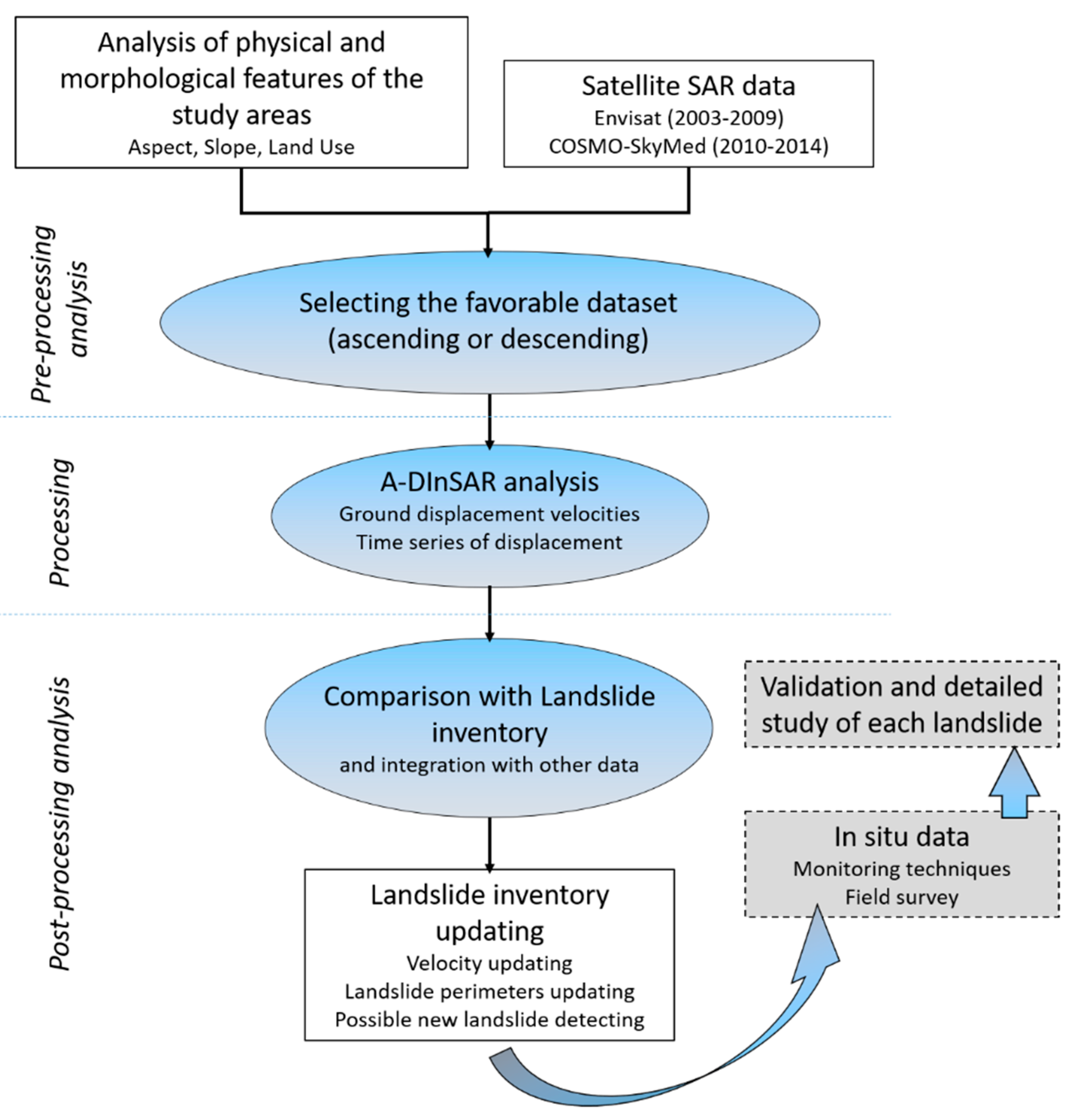
3. Materials and Methods

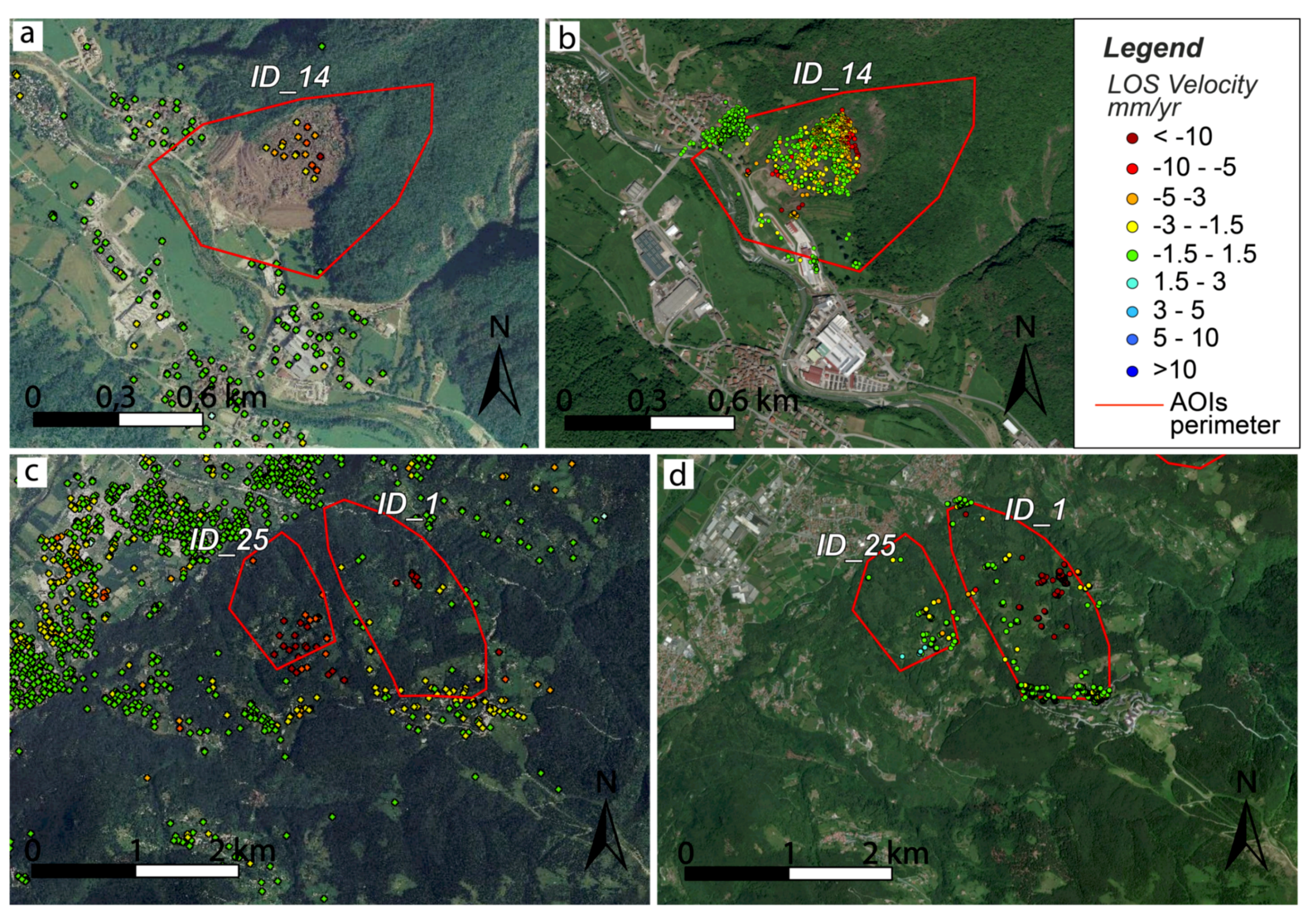
Over the last two decades, classical Differential SAR interferometry (DInSAR) analyses, performed by coupling SAR images to generate differential interferograms have been largely adopted as a tool to investigate ground deformation processes.

This technique exploits the information contained in the phase of the signal of two complex SAR images acquired in different times over the same area, used to form the so-called interferogram [46].

The differential interferogram is formed by subtracting the topographic contributions from the interferometric phase, by using a reference DEM (Digital Elevation Model), thus allowing retrieval of the phase component related to displacement.

The deformation is highlighted by the presence of the so-called “interferometric fringes”. The color cycle of one fringe (from red to blue) corresponds to a displacement of half of the wavelength. Thus, considering the characteristics of the Envisat and COSMO-SkyMed satellites, one fringe corresponds to a displacement of about 2.8 cm and 1.5 cm respectively, in the Line of Sight (LOS) direction.

However, some limitations affect DInSAR, such as artifacts due to the atmosphere phase screen (APS), the presence of residual topographic contributions, and decorrelation effects (both temporal and geometrical), which can prevent the observation of displacement information or reduce the accuracy of the results.

Advanced DInSAR (A-DInSAR) techniques represent an effective solution to reduce some of the limitations of standard DInSAR analysis [27,47,48,49,50]. All A-DInSAR approaches are basically characterized by the exploitation of large, multi-temporal data-stacks to generate several interferograms, thus achieving higher redundancy of interferometric results. One of the most known approaches is the so-called Persistent Scatterers Interferometry (PSI), which is based on the information achieved by pixels of the SAR images characterized by high coherence over long time intervals [27,47,48,50]. Generally, man-made structures, such as buildings, bridges, dams, railways, or pylons, or natural elements, such as outcropping rocks or homogeneous terrain areas, can represent good Persistent Scatterers (PSs).

Standard PSI is based on the generation of interferograms using a common master SAR image. Point-like scattering pixels remain coherent for the whole observation period of time and are not affected by temporal and geometrical decorrelation effects. The interferograms are generated using image pairs characterized by long temporal and normal baselines. Using this principle, almost all images that constitute a given stack can be used to perform multi-temporal A-DInSAR analyses. A collection of images that can be processed together in an A-DInSAR analysis is called an interferometric stack. In order to retrieve the time series of displacement, a minimum number of 15–20 images collected with the same acquisition geometry is required [46], however, the larger the number of available scenes the better the quality of the average velocity estimation and of the time series of displacement.

The general limitations of satellite SAR interferometry are well known in literature [28,51] and are related to methodology of SAR image processing, to the characteristics of space born sensors (geometry of acquisitions, used wavelength, revisiting time) as well as topography and the land use. In fact, the terrain elevation results in geometric distortions in the SAR images [52], and this affects the ground resolution cell. Foreshortening effect cause a “compression” in the slopes that are facing the radar sensor. The so-called layover occurs for the slopes that are inclined away from the sensor with an angle slope higher than the incidence angle of the LOS, i.e., the sensor firstly receives the signal reflected by the top and then the signal coming from the bottom of the slope. Finally, shadow effects occur when an object on the ground prevents the radar signal to reach other ground scatterers and no measurements are possible on those areas. Therefore, the best geometry to detect PSs in mountainous areas is where the slope is parallel to the satellite LOS, e.g., Notti et al. [14].

As regards the limitations of the A-DInSAR due to the land use, this technique is not suitable over highly vegetated areas, or water bodies, as only radar targets that do not change their reflective signature over time can be analyzed.

The A-DInSAR analyses have been performed using 181 COSMO-SkyMed (Italian Space Agency, ASI) images for the time span from 2010 to 2014. The main characteristics of the data and the footprints of the COSMO-SkyMed images are showed in Figure 7.

The time span 2003–2009 is covered by an Envisat (European Space Agency, ESA) data stack. These data were processed in the framework of the Not-Ordinary Plan of Remote Sensing project (promoted by the Italian Ministry of the Environment and for Protection of the Land and Sea) and are available online at the Italian National Geoportal webpage [53]. The use of this source of information in addition to the COSMO-SkyMed data, allowed to exploit a greater number of A-DInSAR results and to get more reliable statistic results. Historical Envisat data were processed with the PSI technique [48], and in the framework of this study, these results have been consulted on the Geoportal webpage. COSMO-SkyMed stacks were processed with the multi-temporal A-DInSAR interferometric processing, including PSI [47,54] for the aims of this work.For one of the AOIs (ID_13) no satellite data were available, and for ID_12 and ID_20 only Envisat data were present.

In Figure 8, a flowchart showing the different main steps and aims of the study is represented. The used methodology belongs to a comprehensive A-DInSAR study and can be resumed as follows: (i) The pre-processing phase, (ii) the processing and (iii) the post-processing analysis.

(i) The pre-processing phase focused on the prediction of PSs distribution, by observing the physical characteristics of the AOIs, such as the land use, the aspect and the slope angles of the mountain and hilly regions where the 26 AOIs are located. This step lead to the selection of the most favorable dataset (ascending or descending) respect to the investigated slopes.

(ii) The A-DInSAR processing phase allows to generate velocity maps and time series of displacement of radar targets (measurement points or PSs). Processing is aimed to reduce the effects of spatial and temporal decorrelation, thus increasing the number of reliable measurement points. Moreover, the performed workflow has been adapted to the specific cases, the characteristics of the AOIs and the evolution of observed processes. A reference point (zero deformation points) was selected for each AOIs, considering the phase stability of the PS candidates.

The main features and of the Envisat and COSMO-SkyMed data and results are resumed in

Table 1. SAR data used in this work and general processing results.

Satellite	Envisat	COSMO-SkyMed
Sensor’s band	C-band	X-band
Acquisition geometry	Asc. + Desc.	Asc. + Desc.
Look angle (°)	23	34
Time span	2003–2009	2010–2014
No of images	-	181
No of PSs for Asc. (sum of AOIs)	417	6753
No of PSs for Desc. (sum of AOIs)	873	5545
Mean PS density for Asc. (PS/km2)	27.3	526.1
Mean PS density for Desc. (PS/km2)	46.1	525.8
Velocity range for Asc. (max; min) (mm/yr)	−5.10; 0.24	−10.77; 0.34
Velocity range for Desc. (max; min) (mm/yr)	−12.91; 0.61	−7.35; 3.06

. The Envisat and COSMO-SkyMed radar targets are detected with different amounts, distribution and density. This is mainly due to the different characteristic of the sensors: Envisat had medium spatial resolution (~25 m) sensor, operating in C band (wavelength = 5.6 cm), while COSMO-SkyMed satellites are equipped with high-resolution (~3 m) sensors, operating in X-band (wavelength = 3.1 cm). Sensors with short wavelengths (X-band) can detect smaller scatterers and provides a higher spatial resolution and increases the PS density.

(iii) The post-processing step consisted in the comparison in GIS environment of the A-DInSAR results with the IFFI landslide inventory, in order to update the landslide inventory and in particular the state of activity of the landslides that occur within the AOIs.

4. Results

The outputs of this work result from the different steps belonging to a comprehensive A-DInSAR study: (i) The pre-processing phase, (ii) the A-DInSAR processing, and (iii) the post-processing analysis.

(i) Pre-processing phase. As stated before, A-DInSAR allows to select PSs over objects like buildings, infrastructures, or rocks, that provide a stable electromagnetic response to the satellite radar signal, during the whole monitoring period. As shown in Figure 6, the land use is in general not favorable for detecting persistent scatterers, as vegetated areas represent about the 90% of the territory, while the urbanized zones are poorly represented in the AOIs territories.

The aspect and slope maps have been extracted from a DEM (Digital Elevation Model) in a GIS (Geographic Information System) environment and the values were classified according to the classes shown in Figure 9. As regards the aspect, most AOIs look towards the western quadrant (7 AOIs are faced to SSW-SW and 8 AOIs are oriented about towards W). As regard the slope, the 65% of the AOIs are characterized by angles between 18° and 32°, while 6 AOIs are gently inclined (slope lower than 18°) and only 3 are located on very inclined slopes (>32°).

(ii) A-DInSAR processing. For the aim of this work, A-DInSAR processing provided two main results: the number (and therefore the density) of radar reflectors (PSs) and the mean LOS velocity values of each radar reflectors.

The PSs coverage for Envisat and COSMO-SkyMed satellites is described in Table 1 where the number of PSs is showed as the total sum for all the investigated AOIs. In

Table 2. Number of PSs and PSs density (PSs/Km²) resulting from A-DInSAR analysis for each AOIs. Red values indicate N. of PSs <10. The last two columns summarize the aspect and slope classes described in Figure 9 for each AOIs.

AOIS		ENVISAT (2003–2009)				COSMO-SkyMed (2010–2014)				ASPECT (°)		SLOPE (°)
ID	Name	N. of PSs (Desc.)	PSs/Km2 (Desc.)	N. of PSs (Asc.)	PSs/Km2 (Asc.)	N. of PSs (Desc.)	PSs/Km2 (Desc.)	N. of PSs (Asc.)	PSs/Km2 (Asc.)
ID_1	ACQUEBUONE	90	33.43	/	/	/	/	848	314.96	0–22.5	N–NNE	18–25
ID_2	POPOIA	27	48.66	20	36.05	/	/	375	675.88	202.5–225	SSW–SW	18–25
ID_3	VAL VEDETTA	4	7.17	/	/	/	/	15	26.88	292–315.5	WNW–NW	25–32
ID_4	GIUBEZZA	4	5.20	49	62.02	/	/	938	1187.20	112.5–135	ESE–SE	11–18
ID_5	PAISCO LOVENO	/	/	25	34.60	/	/	505	698.97	157.5–180	SSE–S	18–25
ID_6	GRUMELLO	/	/	13	12.21	/	/	250	234.72	157.5–181	SSE–S	25–32
ID_7	TROBIOLO	12	19.33	1	1.61	/	/	420	676.49	292.5–315	WNW–NW	32–39
ID_8	ZINVILL	/	/	20	27.64	/	/	561	775.38	112.5–135	ESE–SE	32–39
ID_9	DOSSENA	78	136.62	31	54.30	/	/	945	1655.24	202.5–225	SSW–SW	18–25
ID_10	PAGAFONE	143	98.96	58	40.14	/	/	1481	1024.85	202.5–225	SSW–SW	11–18
ID_11	CATASCO	40	45.09	83	93.56	1362	1535.27	/	/	157.5–180	SSE–S	18–25
ID_12	SAN NAZZARO	78	157.12	16	32.23	/	/	/	/	202.5–225	SSW–SW	25–32
ID_13	BEDOLESSO	/	/	/	/	/	/	/	/	0–22.5	N–NNE	25–32
ID_14	CORTENOVA	28	21.56	/	/	987	760.10	77	59.30	225–247.5	SW–WSW	18–25
ID_15	GARAVINA	16	20.59	6	7.72	91	117.12	102	131.28	0–22.5	N–NNE	25–32
ID_16	TORRIONI Di R.	14	34.32	/	/	239	585.96	/	/	202.5–225	SW–WSW	46–53
ID_17	RONCO	3	17.86	/	/	24	222.88	5	16.43	0–22.5	N–NNE	18–25
ID_18	SASSO DEL PEC.	3	1.10	35	12.81	163	59.65	355	129.92	67.5–90	ENE–E	11–18
ID_19	GERO BARCONE	65	72.31	15	16.69	990	1101.33	644	716.42	202.5–225	SSW–SW	25–32
ID_20	GANDELLINO	38	27.38	/	/	/	/	/	/	247.5–270	WSW–W	25–32
ID_21	SORIASCO	25	77.48	13	40.29	228	706.59	/	/	202.5–225	SSW–SW	4–11
ID_22	RUINELLO	51	23.29	29	13.24	511	233.38	/	/	112.5–135	ESE–SE	4–11
ID_23	VIGNOLA	4	17.37	/	/	23	214.86	/	/	202.5–225	SSW–SW	18–25
ID_24	POGGIO FER.	11	25.21	1	2.80	116	324.96	/	/	270–292.5	W–WNW	11–18
ID_25	RONCAGLIA	29	18.17	2	1.25	/	/	102	63.91	292.5–315	WNW–NW	18–25
ID_26	NOCENO	22	34.71	/	/	284	448.11	/	/	225–247.5	SW–WSW	25–32

, the number of PSs and the related density (PSs/Km²) are showed for each AOIs. These values are significantly higher for the COSMO-SkyMed data, mainly due to the better resolution described in the previous paragraph. In general, the higher the PSs number, the more reliable the results are. An arbitrary minimum threshold of 10 PSs has been set, in order to discard the cases (highlighted in red in Table 2) where very few PSs have been detected. Below this threshold, the results will not be considered as reliable and will not be used in the following work steps.

The mean deformation rates in millimeter per year for each AOIs and the related standard deviation values are reported in

Table 3. Summary and statistics of the A-DInSAR results with respective reference years, and the related updating of landslide inventory (IFFI, 2007). State of activity categories of the IFFI inventory: (A) activated, reactivated, suspended; (Un) undefined; (Q) quiescent. Vlos DESC: Velocity (LOS direction) of the descending dataset; Vlos ASC: Velocity (LOS direction) of the ascending dataset; σ (Vlos): standard deviation of the velocity values. Red x: not reliable velocity values, i.e., values calculated on a N° PS ≤10; slash: satellite data not available. Green: possibility to update the inventory; yellow: reliable data but insufficient information to update the inventory; red: data not available or failure to update inventory.

AOIs		Literature Information			Envisat (2003-2009)				COSMO-SkyMed (2010-2014)				Landslide Inventory Updating				State of Activity Updating
ID	Name	Area (km2)	% Area Affected by Landslide	Sate of Activity (IFFI)	VLOS Desc. (mm/yr)	σ (VLOS Desc.)	VLOS Asc. (mm/yr)	σ (VLOS Asc.)	VLOS Desc. (mm/yr)	σ (VLOS Desc.)	VLOS Asc. (mm/yr)	σ (VLOS Asc.)	Velocity	Landslide Perimeter	Possible New landslides
ID_1	ACQUEBUONE	2.70	100.0	Un.	−3.04	4.08	/	/	/	/	−10.77	0.59	yes	yes	yes		yes
ID_2	POPOIA	0.55	14.4	A	0.61	0.42	0.13	0.40	/	/	0.34	0.62	yes	no	no		yes
ID_3	VAL VEDETTA	0.70	27.1	Un.	x	x	/	/	/	/	−1.17	0.98	yes	no	no		no
ID_4	GIUBEZZA	0.79	39.2	Un.	x	x	0.02	0.46	/	/	0.23	1.02	yes	no	no		yes
ID_5	PAISCO LOVENO	0.72	14.4	A	/	/	−2.11	1.18	/	/	−3.46	0.58	yes	yes	no		yes
ID_6	GRUMELLO	1.10	29.1	Un.	/	/	−0.55	0.43	/	/	−0.17	1.58	yes	yes	yes		yes
ID_7	TROBIOLO	0.62	38.7	Q	−0.02	2.18	x	x	/	/	−0.38	0.58	yes	no	no		no
ID_8	ZINVILL	0.76	62.5	Un.	/	/	−3.04	1.30	/	/	−5.54	0.60	yes	yes	yes		yes
ID_9	DOSSENA	0.24	42.1	Un.	−2.11	2.00	−0.48	0.66	/	/	−1.90	0.47	yes	no	no		yes
ID_10	PAGAFONE	1.40	100.0	Un.	−4.07	1.42	−0.77	0.75	/	/	−2.44	0.47	yes	no	yes		yes
ID_11	CATASCO	0.89	98.9	Un.	−1.72	1.67	−5.10	1.79	−3.12	0.37	/	/	yes	yes	yes		yes
ID_12	SAN NAZZARO	0.50	14.0	Un.	−0.48	1.02	−0.50	0.83	/	/	/	/	yes	no	no		no
ID_13	BEDOLESSO	1.60	100.0	Un.	/	/	/	/	/	/	/	/	no	no	no		no
ID_14	CORTENOVA	1.30	26.9	Un.	−4.28	4.16	/	/	−3.31	0.40	−0.52	1.43	yes	yes	yes		yes
ID_15	GARAVINA	0.78	100.0	Un.	−5.59	1.74	x	x	−6.18	0.43	−4.99	0.47	yes	yes	no		yes
ID_16	TORRIONI Di R.	0.41	75.6	Un.	−0.13	0.59	/	/	−2.74	0.42	/	/	yes	yes	yes		yes
ID_17	RONCO	0.11	100.0	Un.	x	x	/	/	−0.59	0.53	x	x	yes	no	no		no
ID_18	SASSO DEL PEC.	2.70	28.5	Un.	x	x	−0.32	0.60	−0.25	0.54	−0.72	0.46	yes	no	no		yes
ID_19	GERO BARCONE	0.90	81.1	Un.	0.36	0.52	−0.24	0.35	−0.22	0.59	0.09	0.63	yes	no	no		yes
ID_20	GANDELLINO	1.40	67.9	Un.	−5.04	2.62	/	/	/	/	/	/	yes	yes	no		no
ID_21	SORIASCO	0.32	20.6	Q	−0.53	0.96	−0.28	0.71	−0.23	0.74	/	/	yes	no	no		yes
ID_22	RUINELLO	2.20	63.6	Q	−0.31	1.33	−1.73	1.62	3.06	0.43	/	/	yes	yes	yes		yes
ID_23	VIGNOLA	0.11	65.5	Q	x	x	/	/	−0.72	0.75	/	/	yes	no	no		no
ID_24	POGGIO FER.	0.36	50.0	A	−3.68	4.12	x	x	−7.35	0.46	/	/	yes	yes	yes		yes
ID_25	RONCAGLIA	1.60	100.0	Un.	−12.91	4.55	x	x	/	/	-2.50	0.58	yes	no	no		no
ID_26	NOCENO	0.63	15.9	Un.	−0.41	1.62	/	/	−2.77	0.40	/	/	yes	yes	no		yes

. Given the sensitivity of the sensor and the standard deviation analysis of the velocity values for the stable areas, the velocities among −1.5 and 1.5 mm/yr have been considered as not moving. As stated in the previous paragraph, the perimeter of each AOI doesn’t correspond entirely to a landslide but can also include stable zones. For this reason, the mean velocity values of Table 3 have been calculated in subsets of PSs selected on zones that showed deformation (i.e., velocity < −1.5 or > 1.5).

The velocity values have been considered reliable when are retrieved on a PSs number >10. The cases below this threshold, have not be considered for the interpretation of results and are represented with a red x in Table 3.

Some examples regarding the spatial distribution of A-DInSAR results derived from COSMO-SkyMed and Envisat sensors are shown in Figure 10, where three AOIs and their maps of displacement are represented. The PSs characterized by negative velocity values (in red colors) are moving away from the sensor, while PSs with positive velocities (in blue) are moving towards the sensor. The PSs with velocity among −1.5 and 1.5 mm/yr (green color) have been considered as stable.

(iii) Post-processing analysis. The landslide inventory can be updated through three different specific information deduced by A-DInSAR results interpretation, that are: (1) A reliable velocity value of the landslide for the analyzed time span; (2) the redefinition of the landslide boundary; (3) the detection of new deformation phenomena. For each AOIs, the possibility to retrieve this information is summarized in the last 4 columns of the Table 3. The colors of velocity and of the state of activity columns are described in the discussion.

5. Discussion

The results of this work provide the opportunity to verify how the satellite SAR acquisition geometry and the morphological characteristics of the AOIs (land use, slope angle, slope dip orientation) affect the PSs coverage and the performance of A-DInSAR technique, by using 26 case studies (AOIs) in Lombardy region. Moreover, this work allows to consider the success rate of A-DInSAR analysis for updating landslide inventory in such mountainous region, with a limited set of available satellite SAR data.

As only relatively slow landslides (<100 mm/yr) can be detected and monitored effectively by PSI analysis, the AOIs of Lombardy Region have been selected in zones affected by rotational/translational slides and by deep-seated gravitational slope deformations (DSGSD). In general, for the other type of landslides (i.e., rock fall) the PSI data maybe in some cases considered as precursor of rupture [31], but usually are not suitable for analyze fast processes.

The land use strongly influences the detection of stable reflectors (rocks and debris, buildings or other infrastructures, like pylons, railways, etc.), and in our study this represented and important limitation for all the case studies (more than 80% of the territory of interest is covered by Forest Land: 60.6% and Grassland: 22.4%). For this reason, in fact, in some cases only a few PSs have been identified and this was not considered enough to assess the velocity of the deformation phenomena (if any).

The other typical limitations of satellite SAR interferometry are the geometric distortion effects (layover, foreshortening and shadow effects) that depend upon the slope angle and the slope dip orientation and can prevent the PSs being detected [6,32]. In this regard, we compared the results of Envisat and COSMO-SkyMed, for both ascending and descending acquisition modes and then we analyzed them in relation with the morphology or physical characteristics of the AOIs. Frist of all, we observe that COSMO-SkyMed allows to identify more PSs on the ground with respect to Envisat (it is possible to compare the results of the two datasets in Table 2, where the number and the density of PSs for both Envisat and COSMO-SkyMed are shown). Beside the role played by the different spatial resolutions of the two sensors, also the incidence angle of the satellite LOS can influence the effectiveness of the technique. In fact, the use of a high incidence angle (e.g., 34°) of COSMO-SkyMed, reduces layover and foreshortening with a little increase in the shadowing effect, and can better detect movements with a significant horizontal component (in particular in E-W direction).

In Table 2, the number of PSs for each AOIs is compared with the aspect and the slope. It is worth to note that the AOIs with aspect about north and south are characterized by a limited number of PSs, for all the data-stacks.

Moreover, in general, the satellite acquisition geometry is not favorably oriented to retrieve measurement in north-south direction, both for ascending and descending modes, as SAR satellites have a quasi-polar orbit and a right looking. In fact, SAR sensor can only measure deformation along the LOS direction: Only the component of the movement projected along the LOS can be measured. The slopes with aspect towards north or south can’t be projected along the LOS as are approximately parallel.

For the same reason, ascending geometry is favorable for analyzing slopes with aspect towards west, obtaining many measurement points, whereas the ascending geometry works better for slopes facing to the east [33]. For the AOIs analyzed with both ascending and descending datasets, has been possible to verify the effectiveness of both acquisition geometries, according to the AOI’s aspect. The comparison of the two results has been possible for 19 cases: 14 couples of geometries for Envisat and 5 for COSMO-SkyMed (as showed in

Table 4. Comparison of the A-DInSAR results for the AOIs analyzed with both ascending and descending datasets. Green color indicates the cases in which the descending geometry retrieves a larger number of PSs on slopes with aspect towards west, and cases in which the ascending geometry retrieves a larger number of PSs on slopes with aspect towards east. Red color indicates the cases where the comparison of results doesn’t confirm this general trend about SAR acquisition geometries.

AOIs		Envisat (2003–2009)				Aspect (°)		Slope (°)
ID	Name	No PSs (desc)	PSs density (PS/km2)	N°PSs (asc)	PSs density (PS/km2)
ID_2	POPOIA	27	48.66	20	36.05	202.5–225	SSW-SW	18–25
ID_4	GIUBEZZA	4	5.20	49	62.02	112.5–135	ESE-SE	11–18
ID_7	TROBIOLO	12	19.33	1	1.61	292.5–315	WNW-NW	32–39
ID_9	DOSSENA	78	136.62	31	54.30	202.5–225	SSW-SW	18–25
ID_10	PAGAFONE	143	98.96	58	40.14	202.5–225	SSW-SW	11–18
ID_11	CATASCO	40	45.09	83	93.56	157.5–180	SSE-S	18–25
ID_12	SAN NAZZARO	78	157.12	16	32.23	202.5–225	SSW-SW	25–32
ID_15	GARAVINA	16	20.59	6	7.72	0–22.5	N-NNE	25–32
ID_18	SASSO DEL PEC.	3	1.10	35	12.81	67.5–90	ENE-E	11–18
ID_19	GERO BARCONE	65	72.31	15	16.69	202.5–225	SSW-SW	25–32
ID_21	SORIASCO	25	77.48	13	40.29	202.5–225	SSW-SW	4–11
ID_22	RUINELLO	51	23.29	29	13.24	112.5-135	ESE-SE	4-11
ID_24	POGGIO FER.	9	25.21	1	2.80	270-292.5	W-WNW	11-18
ID_25	RONCAGLIA	29	18.17	2	1.25	292.5-315	WNW-NW	18-25
AOIs		COSMO-SkyMed (2010–2014)				Aspect (°)		Slope (°)
ID	Name	N° PSs (desc)	PSs density (PS/km2)	N°PSs (asc)	PSs density (PS/km2)
ID_14	CORTENOVA	987	760.10	77	59.30	225–247.5	SW-WSW	18–25
ID_15	GARAVINA	91	117.12	102	131.28	0–22.5	N-NNE	25–32
ID_17	RONCO	24	222.88	5	46.43	0–22.5	N-NNE	18–25
ID_18	SASSO DEL PEC.	163	59.65	355	129.92	67.5–90	ENE-E	11–18
ID_19	GERO BARCONE	990	1101.33	644	716.42	202.5–225	SSW-SW	25–32

). The general rule of SAR acquisition geometry can be confirmed in most cases: 16 AOIs among 19 (in green in Table 4), i.e., about the 84% of the cases analyzed with ascending and descending.

This is highlighted in the histograms of Figure 11, where the number of PSs of COSMO-SkyMed and Envisat data-stacks is showed with the aspect for each AOIs. In the horizontal axis, the AOIs are ordered according to the aspect direction, from north in a clockwise direction (east and west are ideally indicated in the histogram). As stated before, generally for aspect facing east (left side of the histograms) the results of descending dataset allow to retrieve a larger number of PSs, and for aspect facing west (right side of the histograms), the results of ascending dataset allow to retrieve a larger number of PSs. The results that don’t confirm this general outcome (i.e., the cases in which were collected more PSs by the theoretically unfavorable acquisition geometry) are highlighted by black ellipsis in the histograms, the same cases indicated in red in Table 4 and correspond to one case of the COSMO SkyMed dataset (ID_17), and two cases of the Envisat dataset (ID_15 and ID_22). This could be due to typical characteristics of the study areas, as slope and aspect are not uniform in a natural slope, determining peculiar settings, roughness and counterslopes. Therefore, many PSs can be retrieved in some small sectors of the AOI with peculiar condition of slope and aspect [7], which can assume favorable orientation. Moreover, a very low slope angle (topography almost flat) can practically eliminate the influence of the aspect.

Several predictive models to improve the use of Persistent Scatterers (PSs) techniques for landslides study and to forecast the potential PSs distribution have been proposed in the past years [7,12,30,34,35,51,55]. The natural roughness, the variability of the slope topography and orientation and the big number of features that can affect the radar signal response in a hilly and mountainous region, as for example the occurrence of vegetated areas or the roughness caused by man-made structures, make it difficult to apply predictive model reliably. In general, the use of both descending and ascending geometries, can prevent problems of lack of measurement points in slopes and in complex and steep ground morphologies, and is useful to retrieve the real displacement vector of a landslide. However, a preliminary study of a large number of landslides can benefit of a single-geometry A-DInSAR study: The pre-processing analysis of the aspect setting, can guide the selection of the better oriented satellite geometry, ensuring a greater amount of measurement points. In this study, indeed, we observe that the expected favorable geometry (i.e., ascending for slopes facing east and descending for slopes facing west) provided a more reliable result in about the 84% of the case studies.

As confirmed in several works, A-DInSAR analysis can be used for landslide inventories updating and can be integrated with field surveys and conventional thematic data for a correct results application and interpretation. In this work, the A-DInSAR outputs allowed to observe several zones affected by active landslides, and therefore to validate and update the landslide inventory. Several landslides considered as active, reactivated or suspended have been confirmed to be affected by deformation while, in other cases, new deformation phenomena have been detected. An example is showed in Figure 12: The velocity values of some PSs of ID_1 are up to −10 mm/yr (red color), showing that the landslide is probably active during the time span of COSMO-SkyMed data. Moreover, the landslide perimeter could be re-drawn according to the PSs velocity.

Based on similar considerations for each area of study, this work had the purpose of detailing and quantifying the new data provided by A-DInSAR analysis. Compared to other works of literature such as [33], we specify which kind of information can be updated on each AOIs: the velocity value, the landslide perimeters, the detection of new landslides. As introduced in the previous paragraph, this information is summarized in the last 4 columns of the Table 3, and the “velocity” and the “state of activity” are highlighted with colors in order to show the effectiveness and the quality of the results, and in particular: Green correspond to reliable values, with possibility to update the landslide inventory; yellow represents reliable data, but the retrieved information is not robust enough to update the inventory; red indicates that the satellite data was not available or that the results can’t update the inventory. In most of the cases, when a reliable velocity value is obtained but it is indicated in yellow in the column of “velocity”, it means that the retrieved velocity measurements are not optimally distributed in the area of interest. This is commonly due to the land use of these AOIs, characterized by forest or grassland, where PSs are concentrated only on small urbanized areas on the edges of the AOIs or on isolated buildings. Therefore, the A-DInSAR technique worked in principle but cannot be used for studying the landslides of interest. Consequently, the velocity values in yellow not allow to update the state of activity of the landslide inventory and this is indicated in red in the last column of Table 3.

The landslides perimeters can be updated and modified thanks to the A-DInSAR results. In particular, this is possible when some moving PSs lay over the same slope, outside and near the perimeter of the previously mapped landslides. An example can be represented by some red PSs in the middle of AOI ID_1 (Figure 12): Here, the previously mapped IFFI polygons could be reviewed following the A-DInSAR results, thus including also the area where the red PSs just outside the landslide boundary are located.

The “possible new landslides” are considered in this work, as deformation zones that lay inside the AOIs boundaries, but that are not included in a previously mapped landslide of IFFI catalogue. In addition, these new detected deformation zones, are not so near, nor in the same slope of the previously mapped landslides and should not lead to a modification of the perimeter, but rather to hypothesize a new landslide.

The retrieved velocity values are technically reliable for all the case studies, except for ID_13 (for which there was no satellite data available). The perimeters of the landslides can be updated for 12 AOIs and 9 new landslides can be inferred. In conclusion, A-DInSAR results can update the state of activity of the previously mapped landslide on 18 cases among 26 (i.e., about 69%), providing new qualitative and quantitative data.

6. Conclusions

This work focused on the capabilities of the A-DInSAR technique and on the optimization of its performances for studying slow-moving landslides, considering some limitations that typically affect wooded and mountainous region.

On a sample of 26 areas of interest in Lombardy Region (Italy), analyzed through A-DInSAR technique, the following conclusions have been drawn:

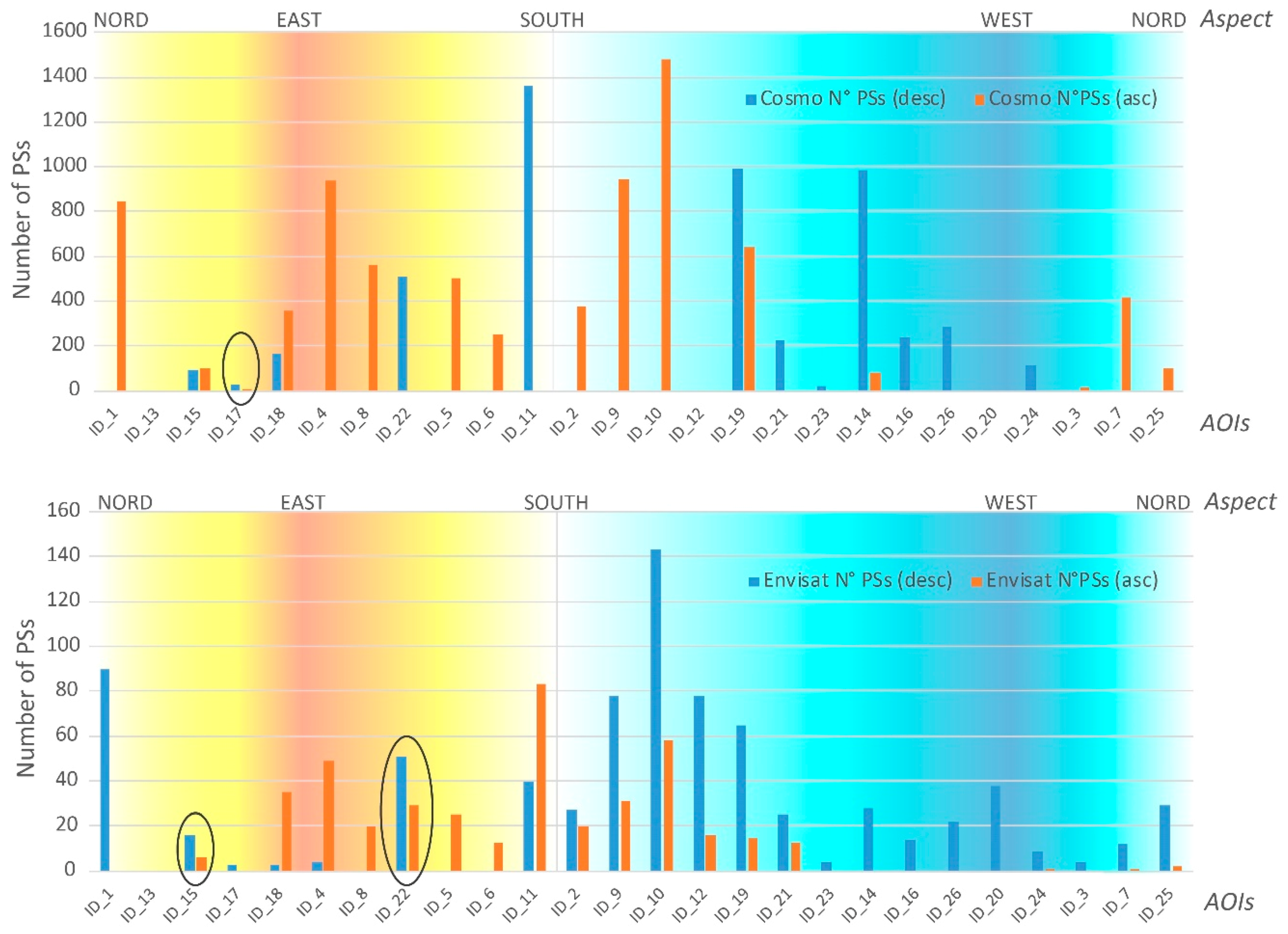
• A-DInSAR analysis in single acquisition geometry, can work properly if the favorable geometry among descending or ascending is chosen with respect to the slope orientation the aspect of the study areas. The single geometry analysis can be successfully applied for the preliminary study of a large number of landslides, or a wide area of interest. About the 16% of information may however be lost, due to the surface irregularity and roughness of the natural slopes. The topographical complexity of the slopes makes the models of prediction of PSs coverage unreliable and the simple rule that ascending acquisition geometry is suitable for E-facing slopes, while descending mode is used for W-facing slopes is not always verified. For detailed studies, indeed, it is recommended to use both SAR acquisition geometries;
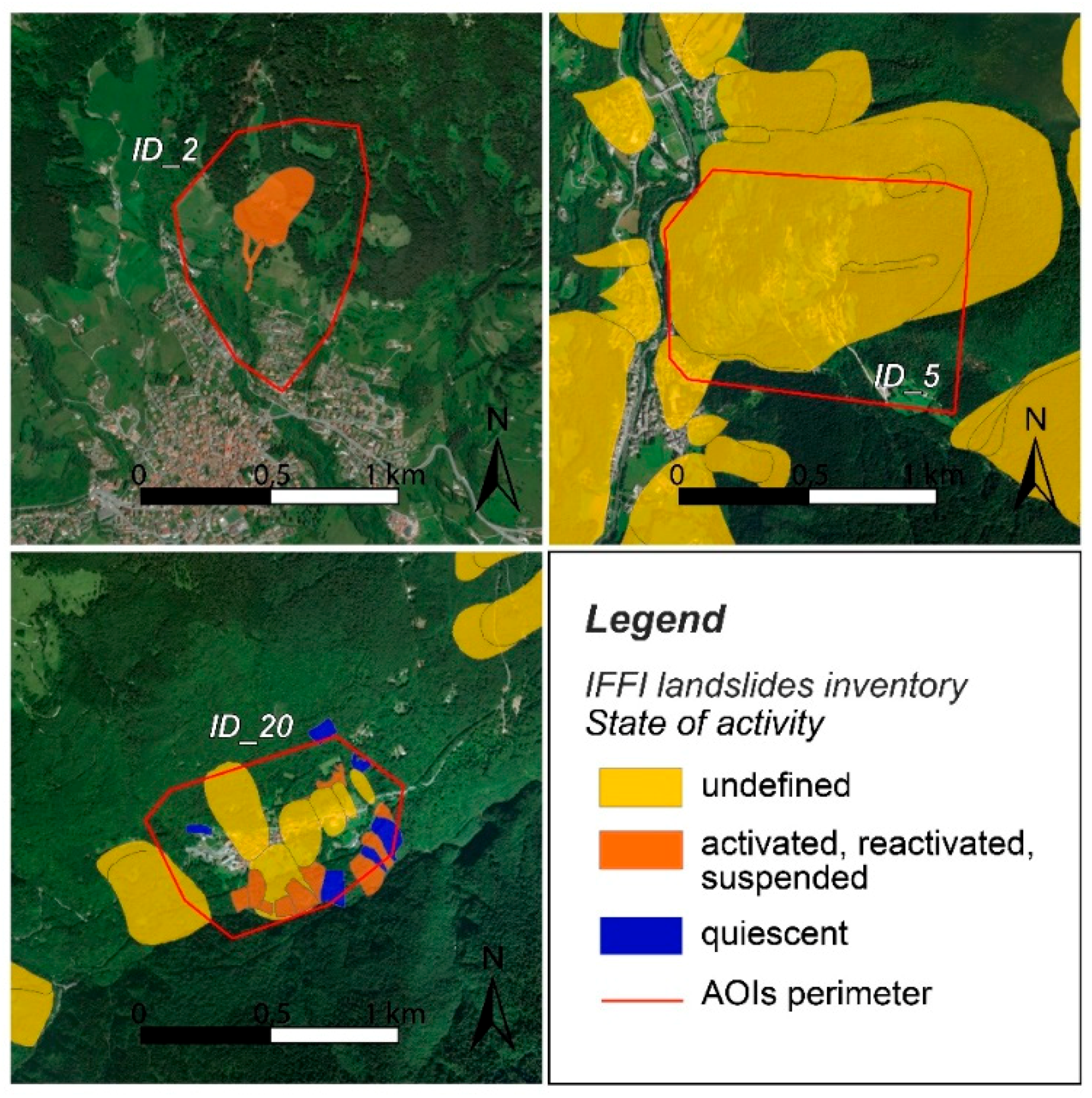
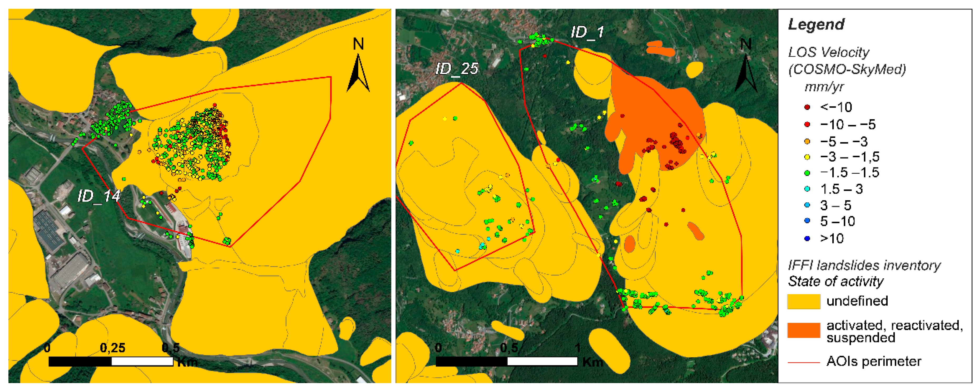
• A-DInSAR outputs can update the state of activity of the previously mapped landslides in about almost 70% of the analyzed areas of interest. In particular, these results provide new qualitative and quantitative data on the landslides, as well as precise information about the velocity of the process, and can redraw the landslide perimeters or detect not previously mapped landslides.

References

1. Varnes, D.J. Landslide Hazard Zonation: A Review of Principles and Practice; Natural Hazard Series; UNESCO: Paris, France, 1984; Volume 3. [Google Scholar]
2. WP/WLI. Working Party on World Landslide Inventory Multilingual Glossary for Landslides; The Canadian Geotechnical Society. BiTech Publisher: Richmond, BC, Cannada, 1993. [Google Scholar]
3. UN-ISDR. Terminology on Disaster Risk Reduction; United Nations, International Strategy for Disaster Reduction: Geneva, Switzerland, May 2019. Available online: http://www.unisdr.org/files/7817_UNISDRTerminologyEnglish.pdf (accessed on 8 May 2019).
4. Corominas, J.; Einstein, H.; Davis, T.; Strom, A.; Zuccaro, G.; Nadim, F.; Verdel, T. Glossary of terms on landslide hazard and risk. In Engineering Geology for Society and Territory; Lollino, G., Giordan, D., Crosta, G.B., Corominas, J., Azzam, R., Wasowski, J., Sciarra, N., Eds.; Springer: Cham, Switzerland, 2015; Volume 2, pp. 1775–1779. [Google Scholar]
5. Meisina, C.; Zucca, F.; Fossati, D.; Ceriani, M.; Allievi, J. Ground deformation monitoring by using the Permanent Scatterers Technique: The example of the Oltrepo Pavese (Lombardia, Italy). Eng. Geol. 2006, 88, 240–259. [Google Scholar] [CrossRef]
6. Colesanti, C.; Wasowski, J. Investigating landslides with space-borne Synthetic Aperture Radar (SAR) interferometry. Eng. Geol. 2006, 88, 173–199. [Google Scholar] [CrossRef]
7. Cascini, L.; Fornaro, G.; Peduto, D. Advanced low- and full-resolution DInSAR map generation for slow-moving landslide analysis at different scales. Eng. Geol. 2010, 112, 29–42. [Google Scholar] [CrossRef]
8. Strozzi, T.; Delaloye, R.; Kääb, A.; Ambrosi, C.; Perruchoud, E.; Wegmuller, U. Combined observations of rock mass movements using satellite SAR interferometry, differential GPS, airborne digital photogrammetry, and airborne photography interpretation. J. Geophys. Res. Space Phys. 2010, 115. [Google Scholar] [CrossRef] [Green Version]
9. Righini, G.; Pancioli, V.; Casagli, N. Updating landslide inventory maps using Persistent Scatterer Interferometry (PSI). Int. J. Remote. Sens. 2011, 33, 2068–2096. [Google Scholar] [CrossRef]
10. Bozzano, F.; Rocca, A. Remote monitoring of deformation using Satellite SAR Interferometry. Geotech. News 2012, 30, 26. [Google Scholar]
11. Cigna, F.; Del Ventisette, C.; Liguori, V.; Casagli, N. Advanced radar-interpretation of InSAR time series for mapping and characterization of geological processes. Nat. Hazards Earth Syst. Sci. 2011, 11, 865–881. [Google Scholar] [CrossRef]
12. Herrera, G.; Gutierrez, F.; García-Davalillo, J.C.; Guerrero, J.; Notti, D.; Galve, J.P.; Fernandez-Merodo, J.A.; Cooksley, G. Multi-sensor advanced DInSAR monitoring of very slow landslides: The Tena Valley case study (Central Spanish Pyrenees). Remote Sens. Environ. 2013, 128, 31–43. [Google Scholar] [CrossRef]
13. Jebur, M.N.; Pradhan, B.; Tehrany, M.S. Using ALOS PALSAR derived high-resolution DInSAR to detect slow-moving landslides in tropical forest: Cameron Highlands, Malaysia. Geomat. Nat. Hazards Risk 2015, 6, 741–759. [Google Scholar] [CrossRef]
14. Notti, D.; Herrera, G.; Bianchini, S.; Meisina, C.; García-Davalillo, J.C.; Zucca, F. A methodology for improving landslide PSI data analysis. Int. J. Remote Sens. 2014, 35, 2186–2214. [Google Scholar]
15. García-Davalillo, J.C.; Herrera, G.; Notti, D.; Strozzi, T.; Álvarez-Fernández, I. DInSAR analysis of ALOS PALSAR images for the assessment of very slow landslides: The Tena Valley case study. Landslides 2014, 11, 225–246. [Google Scholar] [CrossRef]
16. Barra, A.; Monserrat, O.; Mazzanti, P.; Esposito, C.; Crosetto, M.; Mugnozza, G.S. First insights on the potential of Sentinel-1 for landslides detection. Geomat. Nat. Hazards Risk 2016, 7, 1874–1883. [Google Scholar] [CrossRef] [Green Version]
17. Bozzano, F.; Mazzanti, P.; Perissin, D.; Rocca, A.; De Pari, P.; Discenza, M.E. Basin scale assessment of landslides geomorphological setting by advanced InSAR analysis. Remote Sens. 2017, 9, 267. [Google Scholar] [CrossRef]
18. Moretto, S.; Bozzano, F.; Esposito, C.; Mazzanti, P.; Rocca, A. Assessment of landslide pre-failure monitoring and forecasting using satellite SAR interferometry. Geosciences 2017, 7, 36. [Google Scholar] [CrossRef]
19. Zhang, Y.; Meng, X.; Jordan, C.; Novellino, A.; Dijkstra, T.; Chen, G. Investigating slow-moving landslides in the Zhouqu region of China using InSAR time series. Landslides 2018, 15, 1299–1315. [Google Scholar] [CrossRef]
20. Bouali, E.H.; Oommen, T.; Escobar-Wolf, R. Mapping of slow landslides on the Palos Verdes Peninsula using the California landslide inventory and persistent scatterer interferometry. Landslides 2018, 15, 439–452. [Google Scholar] [CrossRef]
21. Journault, J.; Macciotta, R.; Hendry, M.T.; Charbonneau, F.; Huntley, D.; Bobrowsky, P.T. Measuring displacements of the Thompson River valley landslides, south of Ashcroft, BC, Canada, using satellite InSAR. Landslides 2018, 15, 621–636. [Google Scholar] [CrossRef]
22. Varnes, D.J. Slope movements, type and process. In Landslides Analysis and Control; Schuster, R.L., Krizel, R.J., Eds.; Transportation Research Board: Washinghton, DC, USA, 1978; pp. 11–33. [Google Scholar]
23. Varnes, D.J. Landslide types and processes. Landslides Eng. Pract. 1958, 24, 20–47. [Google Scholar]
24. Hungr, O. Some methods of landslide intensity mapping. In Landslide Risk Assessment, Proceedings of the International Workshop on Landslide Risk Assessment, Balkema, Rotterdam, 19–21 February 1997; Cruden, D., Fell, R., Eds.; Routledge: London, UK, 2018; pp. 215–226. [Google Scholar]
25. Lateltin, O.; Haemmig, C.; Raetzo, H.; Bonnard, C. Landslide risk management in Switzerland. Landslides 2005, 2, 313–320. [Google Scholar] [CrossRef]
26. Uzielli, M.; Nadim, F.; Lacasse, S.; Kaynia, A.M. A conceptual framework for quantitative estimation of physical vulnerability to landslides. Eng. Geol. 2008, 102, 251–256. [Google Scholar] [CrossRef]
27. Ferretti, A.; Fumagalli, A.; Novali, F.; Prati, C.; Rocca, F.; Rucci, A. A new algorithm for processing interferometric data-stacks: SqueeSAR. IEEE Trans. Geosci. Remote Sens. 2011, 49, 3460–3470. [Google Scholar] [CrossRef]
28. Crosetto, M.; Monteserrat, O.; Junger, A.; Crippa, B. Persistent scatterer interferometry: Potential and limits. In Proceedings of the ISPRS Workshop on High- Resolution Earth Imaging for Geospatial Information, Hannover, Germany, 2–5 June 2009. [Google Scholar]
29. Perissin, D.; Wang, T. Repeat-Pass SAR interferometry with partially coherent targets. IEEE Trans. Geosci. Remote Sens. 2012, 50, 271–280. [Google Scholar] [CrossRef]
30. Bianchini, S.; Cigna, F.; Righini, G.; Proietti, C.; Casagli, N. Landslide hotspot mapping by means of persistent scatterer interferometry. Environ. Earth Sci. 2012, 67, 1155–1172. [Google Scholar] [CrossRef]
31. Cigna, F.; Bianchini, S.; Casagli, N. How to assess landslide activity and intensity with Persistent Scatterer Interferometry (PSI): The PSI-based matrix approach. Landslides 2013, 10, 267–283. [Google Scholar] [CrossRef]
32. Raspini, F.; Bianchini, S.; Ciampalini, A.; Del Soldato, M.; Solari, L.; Novali, F.; Del Conte, S.; Rucci, A.; Ferretti, A.; Casagli, N. Continuous, semi-automatic monitoring of ground deformation using Sentinel-1 satellites. Sci. Rep. 2018, 8, 7253. [Google Scholar] [CrossRef] [PubMed]
33. Farina, P.; Colombo, D.; Fumagalli, A.; Marks, F.; Moretti, S. Permanent Scatterers for landslide investigations: outcomes from the ESA-SLAM project. Eng. Geol. 2006, 88, 200–217. [Google Scholar] [CrossRef]
34. Herrera, G.; Notti, D.; García-Davalillo, J.C.; Mora, O.; Cooksley, G.; Sánchez, M.; Arnaud, A.; Crosetto, M. Landslides analysis with C- and X-band satellite SAR data: The Portalet landslide area. Landslides 2011, 8, 195–206. [Google Scholar] [CrossRef]
35. Notti, D.; Davalillo, J.C.; Herrera, G.; Mora, O. Assessment of the performance of X-band satellite radar data for landslide mapping and monitoring: Upper Tena Valley case study. Nat. Hazards Earth Syst. Sci. 2010, 10, 1865–1875. [Google Scholar] [CrossRef]
36. Colombo, A.; Mallen, L.; Pispico, R.; Giannico, C.; Bianchi, M.; Savio, G. Mappatura regionale delle aree monitorabili mediante l’uso della tecnica PS. In Proceedings of the 10th National Conference ASITA, Bolzano, Italy, 14–17 November 2006. ISBN/ISSN:88-900943-0-3-2006. [Google Scholar]
37. Dei Cas, L. Complementarietà fra i dati dell’interferometria satellitare e quelli ottenuti con strumentazione a terra sui versanti in dissesto. Rend. Online Soc. Geol. Ital. 2017, 42, 18–22. [Google Scholar] [CrossRef]
38. Istituto Superiore per la Protezione e Ricerca Ambientale. Progetto IFFI-Inventario dei Fenomeni Franosi in Italia 2007. Available online: http://www.isprambiente.gov.it/it/progetti/suolo-e-territorio-1/iffi-inventario-dei-fenomeni-franosi-in-italia / (accessed on 8 May 2019).
39. Trigila, A. Rapporto sulle Frane in Italia: Progetto IFFI metodologia, risultati e rapporti regionali; Agenzia per la protezione dell’ambiente e per i servizi tecnici, APAT, Rapporti 78; 2007; 681p. Available online: http://www.isprambiente.gov.it/files/pubblicazioni/rapporti/rapporto-frane-2007/4169_Rapporto_2007_78.pdf (accessed on 20 August 2019).
40. Regione Lombardia. Frane Di Lombardia - Centri Abitati e Infrastrutture a Rischio Frana in Lombardia. Inventario Fenomeni Franosi Lombardia (IFFI). 2012. Available online: http://www.geoportale.regione.lombardia.it (accessed on 13 May 2019).
41. Dal Piaz, G.V.; Bistacchi, A.; Massironi, M. Geological outline of the Alps. Episodes 2003, 26, 175–180. [Google Scholar] [Green Version]
42. Berra, F.; Carminati, E. Subsidence history from backstripping analysis of the Permo-Mesozoic succession of the Central Southern Alps (Northern Italy). Basin Res. 2009, 22, 952–975. [Google Scholar] [CrossRef]
43. Carelli, M.; Ceriani, M.; Valbuzzi, E. Analisi del dissesto da frana in Lombardia. In Rapporto sulle Frane in Italia: Progetto IFFI metodologia, risultati e rapporti regionali; Trigila, A., Ed.; APAT, 2007. Available online: http://www.isprambiente.gov.it/files/pubblicazioni/rapporti/rapporto-frane-2007/Capitolo_7_Lombardia.pdf (accessed on 20 August 2019).
44. Braga, G.; Braschi, G.; Calculli, S.; Caucia, F.; Cerro, A.; Colleselli, F.; Grisolia, M.; Piccio, A.; Rossetti, R.; Setti, M.; et al. I fenomeni franosi nell'Oltrepo Pavese: tipologia e cause. Geol. Appl. Idrogeol. 1985, 20, 621–666. [Google Scholar]
45. Handy, M.R.; Schmid, S.M.; Bousquet, R.; Kissling, E.; Bernoulli, D. Reconciling plate-tectonic reconstructions of Alpine Tethys with the geological–geophysical record of spreading and subduction in the Alps. Earth-Sci. Rev. 2010, 102, 121–158. [Google Scholar] [CrossRef]
46. Crosetto, M.; Monserrat, O.; Cuevas-González, M.; Devanthéry, N.; Crippa, B. Persistent Scatterer Interferometry: A review. ISPRS J. Photogramm. Remote Sens. 2016, 115, 78–89. [Google Scholar] [CrossRef] [Green Version]
47. Kampes, B.M. Radar Interferometry Persistent Scatterers Technique; Springer: Dordrecht, The Netherlands, 2006. [Google Scholar]
48. Ferretti, A.; Prati, C.; Rocca, F. Permanent scatterers in SAR interferometry. IEEE Trans. Geosci. Remote. Sens. 2001, 39, 8–20. [Google Scholar] [CrossRef]
49. Berardino, P.; Fornaro, G.; Lanari, R.; Sansosti, E. A new algorithm for surface deformation monitoring based on small baseline differential SAR interferograms. IEEE Trans. Geosci. Remote. Sens. 2002, 40, 2375–2383. [Google Scholar] [CrossRef] [Green Version]
50. Hooper, A.; Zebker, H.; Segall, P.; Kampes, B. A new method for measuring deformation on volcanoes and other natural terrains using InSAR persistent scatterers. Geophys. Res. Lett. 2004, 31, 23611. [Google Scholar]
51. Meisina, C.; Zucca, F.; Notti, D.; Colombo, A.; Cucchi, A.; Savio, G.; Giannico, C.; Bianchi, M. Geological interpretation of PSInSAR data at regional scale. Sensors 2008, 8, 7469–7492. [Google Scholar] [CrossRef]
52. Hanssen, R.F. Satellite radar interferometry for deformation monitoring: A priori assessment of feasibility and accuracy. Int. J. Appl. Earth Obs. Geoinformation 2005, 6, 253–260. [Google Scholar] [CrossRef]
53. Italian National Geoportal Webpage, Italian Ministry of the Environment and for Protection of the Land and Sea. Available online: www.pcn.minambiente.it/mattm/en/not-ordinary-plan-of-remote-sensing. (accessed on 4 May 2019).
54. Perissin, D. Interferometric SAR multitemporal processing: techniques and applications. In Multitemporal Remote Sensing; Springer: Cham, Switzerland, 2016; pp. 145–176. [Google Scholar]
55. Lu, P.; Casagli, N.; Catani, F.; Tofani, V. Persistent scatterers interferometry hotspot and cluster analysis (psi-hca) for detection of extremely slow-moving landslides. Int. J. Remote Sens. 2012, 33, 466–489. [Google Scholar] [CrossRef]
Figure 1. (a) Location of the analyzed 26 AOIs. Polygons of the AOIs are in red; (b) location of the Figure 1a (red box) in a schematic sketch of Italy.
Geosciences 09 00364 g001
Figure 2. Tectonic Units of Lombardy Region, Italy (the black line shows the border of the Region); modified form Handy et al. [45]. Reproduced with permission from Elsevier, Earth-Science Reviews; published by Elsevier, 2010.
Geosciences 09 00364 g002
Figure 3. Landslides type in Lombardy Region (Italy). Data from Regione Lombardia, [40] in the framework of IFFI project.
Geosciences 09 00364 g003
Figure 4. Areas of interest (AOIs): Three examples that show different situations as regards the presence of mapped landslides and their state of activity, reported by IFFI catalog [38].
Geosciences 09 00364 g004
Figure 5. Surface affected by mapped landslides (in percentage respect to the total area of the AOI). Data from IFFI Inventory map [40].
Geosciences 09 00364 g005
Figure 6. Categories of land use as respect the total extent of the AOIs.
Geosciences 09 00364 g006
Figure 7. Footprints and characteristics of the COSMO-SkyMed images.
Geosciences 09 00364 g007
Figure 8. Methodology and the main steps of this work: (i) Pre-processing phase, (ii) the processing and (iii) the post-processing analysis. The last two boxes in grey represent the validation phase, that is out the scope of this work.
Geosciences 09 00364 g008
Figure 9. Aspect and Slope Classes for the investigated AOIs. Both Aspect and Slope have been represented through classes with a constant sampling interval of 22.5° and 7° respectively.
Geosciences 09 00364 g009
Figure 10. Examples of A-DInSAR results for Envisat and COSMO-SkyMed datasets; (a,b) Envisat descending and COSMO-SkyMed descending respectively, for the AOI ID_14; (c,d) Envisat descending and COSMO-SkyMed ascending respectively, for the AOIs ID_1 and ID_25. The PS mean velocity values are measured along the satellite LOS. The Envisat data are form the Italian Ministry of the Environment and for Protection of the Land and Sea [53].
Geosciences 09 00364 g010
Figure 11. Number of PSs of COSMO-SkyMed and Envisat data-stacks compared with the aspect directions for each AOIs. The AOIs are ordered with respect to aspect direction, from north in a clockwise direction. Black ellipsis indicates the AOIs where the results don’t confirm the general rule of the SAR acquisition geometries (the same AOIs in red of Table 4).
Geosciences 09 00364 g011
Figure 12. Examples of A-DInSAR results compared with the IFFI landslide inventory. for the AOIs ID_14, ID_1 and ID_25.
Geosciences 09 00364 g012