Article

Spatial and Temporal Variability of Glacier Surface Velocities and Outlet Areas on James Ross Island, Northern Antarctic Peninsula

1
Institut für Geographie, Friedrich-Alexander-Universität Erlangen-Nürnberg, Wetterkreuz 15, 91052 Erlangen, Germany
2
Department of Geography, University of Liège, 3, Clos Mercator, Bat. B11, 4000 Liège, Belgium
3
Instituto Antártico Argentino, 25 de Mayo 1143, 1650 San Martín, Argentina
*
Author to whom correspondence should be addressed.
Geosciences 2019, 9(9), 374; https://doi.org/10.3390/geosciences9090374
Submission received: 3 July 2019 / Revised: 19 August 2019 / Accepted: 23 August 2019 / Published: 28 August 2019
(This article belongs to the Special Issue Remote Sensing of Glaciers and Ice Caps)

Abstract

:
The northern Antarctic Peninsula was affected by a significant warming over the second half of the 20th century and the collapse of several ice shelves. Local climate conditions on James Ross Island on the northeastern coast can differ strongly from the main part of the Antarctic Peninsula. This paper reports the spatial and temporal variability of glacier surface velocities and the area of their outlets throughout James Ross Island, and evaluates potential relationships with atmospheric and oceanic conditions. Velocity estimates were retrieved from intensity feature tracking of scenes from satellite synthetic aperture radar sensors TerraSAR-X and TanDEM-X between 2014 and 2018, which were validated against ground observations. Calving front positions back to 1945 were used to calculate outlet area changes for the glaciers by using a common-box approach. The annual recession rates of almost all investigated glacier calving fronts decelerated for the time periods 2009–2014 and 2014–2018 in comparison to the period 1988–2009, but their velocity patterns differed. Analysis of atmospheric conditions failed to explain the different patterns in velocity and area changes. We suggest a strong influence from local bathymetric conditions. Future investigations of the oceanic conditions would be necessary for a profound understanding of the super-position of different influencing factors.

Graphical Abstract

1. Introduction

The northern Antarctic Peninsula has experienced one of the strongest temperature increases on Earth over the second half of the 20th century [1], which is suspected to have started around the 1930s [2]. However, the local impact of this warming is highly variable, especially between the western and eastern side of the Antarctic Peninsula. One of the longest temperature records in Antarctica, at Faraday/Vernadsky station, reveals an increase at the western side by + 0.052 C a 1 (∼ 2.9 C ) during 1950–2005 [3]. The warming trend in the time period of 1968–2005 has been lower at Bellingshausen station on King George Island ( + 0.028 C a 1 or ∼ 1.0 C ), but higher at Marambio station at the eastern side ( + 0.069 C a 1 or ∼ 2.3 C during 1971–2005) [3]. The location of all stations is shown in Figure 1. Some of the hypothesized consequences of the atmospheric warming process were the collapses of the Larsen A/B and Prince-Gustav channel ice shelves [4,5,6,7].
James Ross Island (JRI) is located on the eastern side of the northern Antarctic Peninsula. Glaciers on the western side of the island formerly discharged into the Prince-Gustav channel ice shelf, which is now open water forming the Röhss Bay (Figure 2). A mass loss of 2.4 Gt a 1 was estimated by differencing digital elevation models and repeat-track laser altimetry between 2001 and 2010 for JRI [8]. The mass loss varies across JRI with the highest loss on the western side ( 1.53 Gt a 1 ), followed by the northern part ( 0.70 Gt a 1 ), and the lowest loss for the south ( 0.24 Gt a 1 ). However, the data coverage for the eastern side was poor such that a higher uncertainty in estimates of mass loss is suspected. When assessing the whole northern Antarctic Peninsula, Scambos et al. [8] observed high rates of decreasing surface elevation for the lower elevation areas of the ice shelves on the eastern side. On the western side, negative rates of elevation change were observed for all glacier elevations. The eastern basins, specifically the ones draining into the embayments formerly occupied by ice shelves, account for 72 % of the mass loss [8]. These differences can be partially explained by lower surface mass balances on the eastern side of the Antarctic Peninsula, including JRI. However, as the high mass loss in western JRI [8] shows, a different spatial pattern of glacier mass loss is possible at smaller spatial scales. The elevation of JRI is not as high as the Antarctic Peninsula, and different climate conditions could prevail. This can cause a varied spatial impact, e.g., of Föhn events, especially at the cliff-separated outlet glaciers.
The local warming trend on the Antarctic Peninsula has reversed since the beginning of the millennium. A cooling trend of 0.47 ± 0.25 C decade 1 was reported for 1999–2014 in contrast to a warming of 0.32 ± 0.20 C decade 1 for 1979–1997 [9]. The cooling is explained by stronger cyclonic conditions in the northern Weddell Sea, associated with a stronger mid-latitude jet [9]. This results in a higher frequency of cold east-to-southerly winds and advection of sea ice towards the east coast of the Antarctic Peninsula. A very low mean air temperature increase of + 0.017 C a 1 is found at Marambio station in the time period 2006–2015 [3].
However, the response to these recent climate changes has not been investigated for most of the glaciers on JRI. Between 2009 and 2015, no clear trend is visible in the cumulative surface mass balances of 0.57 ± 0.67 m w . e . ( water equivalent ) and 0.11 ± 0.37 m w . e . reported for Whisky Glacier and Davies Dome, located on Ulu Peninsula in the northern part of JRI [10]. Mass balance data for Bahia del Diablo on Vega Island (Figure 2) were positive in the years 2013/2014 and 2014/2015 ( + 0.190 m w . e . and + 0.025 m w . e . ), whereas a change to negative values appeared in 2015/2016 and 2016/2017 ( 0.561 m w . e . and 0.380 m w . e . ) [11,12], suggesting a net mass loss in the last years. Data from an ice core on JRI [13] reveal a mean accumulation rate of 0.62 ± 0.14 m w . e . a 1 in the time period 1967–2008 with a variability between ∼ 0.40 m w . e . a 1 and 0.90 m w . e . a 1 . High values up to ∼ 0.90 m w . e . a 1 occurred in the first years after 2000, followed by a decrease to ∼ 0.50 m w . e . a 1 around 2004 and a rise above the mean value in the following years [13]. Depending on the response time, the variations in the above mentioned glacier mass balances could be a result from these deviations in accumulation.
Velocity estimates are available for the Röhss Bay in the time period 2001–2009 [14], and revealed an acceleration in the years after the collapse of the ice shelf. Area estimates from 1988–2009 were published by Davies et al. [15], showing an overall glacier retreat over the whole period with higher rates at the south-eastern part of JRI. Additionally, the location of older glacier calving fronts since 1945 are available from the Antarctic Digital Database (ADD) by the Scientific Committee on Antarctic Research (SCAR) [16], which support the hypothesis of a longer lasting glacier recession. Land-terminating glaciers such as Whiskey Glacier shrank most quickly on JRI between 1988 and 2001, but most of the glaciers on the island are tidewater glaciers [15]. Davies et al. [15] expect further retreat in response to a continued atmospheric warming for low-lying tidewater glaciers on JRI. However, a different response to changes in oceanic temperatures and complex calving processes is possible.
The temperature of the Antarctic Circumpolar Current at 60 S has increased by 0.2 C since the 1950s [15]. Bathymetry and ocean temperature data along the east coast of the Antarctic Peninsula are rare. Thus, recent studies on the role of the ocean warming with regard to glacier or ice shelf retreat are available mainly at the western Antarctic Peninsula [17,18,19].
Considering long-term changes in glacier area and surface velocity on JRI observed in the past (e.g., [14,15]), but also short-term fluctuations detected by in-situ measurements on Gourdon Glacier since 2014, this paper aims to update knowledge on several glaciers throughout JRI by
(1)
providing an extended and updated review of comparable glacier area change on James Ross Island;
(2)
analyzing temporal and spatial variability in ice dynamics between 2014 and 2018; and
(3)
determining potential atmospheric and oceanographic forcing factors.

2. Study Site

In the following section, a detailed overview of the differences in glacier-area estimations on JRI is presented, along with details of glacier response to changes in their geometry, atmospheric and oceanic conditions. This should facilitate the interpretation of the changes in velocity and outlet areas.

2.1. Ice Coverage and Glacier Specifications

JRI is an island covering an area of ∼ 2500 km 2 on the northeastern part of the Antarctic Peninsula (Figure 1). Except for Ulu Peninsula, most areas are nearly completly glaciated. The first estimates of the total glaciated area on JRI are from the 1970s obtained from Kosmos KATE-200 space photographs [5]. Rabassa et al. [20] estimated there to be 138 glaciers with an area of 1989.44 km 2 ( 81.41 % glaciated area). Ferrigno et al. [21] used maps and aerial photographs to estimate ice front changes between 1945 and 2000 with a time step of 5–10 years. Davies et al. [15] calculated areas of 104 glaciers on JRI with total glaciated areas of 2192 ± 136.1 km 2 (1988), 1992.6 km 2 (1997), 1902.4 ± 15.2 km 2 (2001), and 1780.5 ± 86 km 2 (2009, congruent to 75 % glaciated area). Their calculated area losses amounts to 290 ± 15.2 km 2 (1988–2001) and 121.9 ± 15.2 km 2 (2001–2009) with only three glaciers advancing during the study period [15]. Their estimate for 2001–2009 is consistent with values published by the Global Land Ice Measurements from Space (GLIMS) project [22], who indicate an ice loss of 122 km 2 , with 101 km 2 resulting from the disintegration of the ice shelf in the Röhss Bay. However, for the time period 1975–2009, Arigony-Neto et al. [22] estimate 182.3 km 2 (including Röhss Bay), which is significantly less than the combined mass loss between 1988 and 2009 determined by Davies et al. [15].
Due to the bedrock structure of JRI, where resistant volcanic rock overlies soft Cretaceous sediments [23], many glaciers have large, flat accumulation areas on the island’s plateau (mostly > 500 m a . s . l . ( above sea level ) reaching up to about 1600 m a . s . l . at Mount Haddington). The large, low-lying and relative flat glacier termini are mostly separated from the accumulation areas by a sharp change in slope at cirque headwalls or cliffs [15]. The hypsometry class of most glaciers at the Ulu Peninsula are bottom-heavy [24]. In contrast, most glaciers located in the main part of the island draining the large Mount Haddington Ice Cap are top-heavy [15]. In comparison to the northern Antarctic Peninsula, JRI has a very high number of glaciers with mean elevations above 200 m a . s . l . [15]. The mean Equilibrium Line Altitude (ELA) strongly varies between glaciers on Ulu Peninsula (about 100 m a . s . l . ) and glaciers draining from the Mount Haddington Ice Cap (> 800 m a . s . l . ) [15]. The gently sloped glaciers draining the Mount Haddington Ice Cap would be especially vulnerable to a rise in ELA. Therefore, Davies et al. [25] expected further glacier melt, recession, and thinning on JRI in the next century, including the marine-terminating glaciers.

2.2. Atmospheric and Oceanic Conditions

The eastern Antarctic Peninsula is on average 3–5 C colder than the western Antarctic Peninsula at the same latitude [27]. Nevertheless, sporadic Föhn wind conditions with unusually high temperatures can occur on the eastern side. This is because the mountainous topography of the Antarctic Peninsula acts as an orographic barrier. Marshall et al. [28] explained that the higher temperature variability at Esperanza station, with stronger and more frequent Föhn events, is due to faster warm northwesterly winds. These events play a crucial role in controlling the climate at the eastern Antarctic Peninsula because they control surface meltwater production [29,30].
Furthermore, there exists a strong relationship between the atmospheric circulation in the Southern Hemisphere, the surface air temperature and the precipitation [28,31,32]. The Southern Annular Mode (SAM) describes the latitudinal shifts in the mid-latitude jet, and a positive phase is associated with stronger circumpolar westerly winds and a warming of the Antarctic Peninsula [33]. However, no consistent spatial pattern of the impact of the SAM across Antarctica was observed by Marshall et al. [33]. Moreover, the overall relationship between surface air temperatures and the SAM is stronger on the east side of the Peninsula than on the west side [28]. A strong positive SAM was observed during 1979 and 2000 [31]. Long-term trends in the Antarctic circulation show a higher frequency of positive SAM during austral summer (December–February), which could induce warmer and drier atmospheric conditions on JRI [32].
Cook et al. [17] and Morris et al. [27] explain that large glacier area loss in the south of the western Antarctic Peninsula results from higher mid-depth (100–300 m ) ocean temperatures in the Bellingshausen Sea during the 2000s. However, the main oceanic influence on JRI is from the Weddell Sea. Thus, depending on the distribution of warmer oceanic layers the influence on JRI can be different. Bathymetric data in this region is rare, limiting out the ability to extrapolate the work of [17,27] to JRI. Glacier melting is expected to increase linearly or above-linearly with ocean temperature above freezing point [17]. Nevertheless, the impact of temperature variability can be reduced due to sea-ice processes keeping the ocean temperatures near the freezing point. Moreover, small-scale bathymetric features have a strong impact on the mixing with deeper layers [34].

3. Materials and Methods

3.1. Surface Velocities

We used a series of synthetic aperture radar (SAR) images acquired by the TerraSAR-X (TSX) and TanDEM-X (TDX) satellite sensors during 2014–2018. We processed co-registered image pairs with temporal baselines of about 1–3 months using the SAR intensity offset tracking algorithm implemented in the GAMMA remote-sensing software [35]. The algorithm tracks consistent image structures such as crevasses or rocks on the glacier surface within a moving search window and calculates displacements between the two input-images. The size of the tracking window, as well as the step size (distance between tracking measurements) has to be adapted to the local conditions and the data properties. We applied different tracking window sizes (64, 128, 256, and 512 pixel) (corresponding to ∼ 126 m × 58 m , ∼ 251 m × 116 m , ∼ 502 m × 232 m , and ∼ 1004 m × 464 m in azimuth and slant range direction) to account for different glacier speeds as well as surface structures on the plateau and the outlet glaciers. An additional filter algorithm based on a comparison of the magnitude and the alignment of the displacement vector removed the unreasonable values [36,37]. Afterwards, the results from the different window sizes were stacked [37]. While tracking works well on most of the glacier tongues, the surface of the plateau does not have enough features to calculate reliable velocities. Due to some remaining artifacts, mostly near ice cliffs, we additionally restricted our analysis to velocity measurements where a standard deviation of < 0.5 m d 1 was met in a surrounding 21 × 21 pixel moving window (corresponding to ∼ 560 m × 560 m ).
The summed error σ v S U M in the derived velocities was assumed to be the square root of the quadratic sum of two independent error sources, the co-registration error ( σ v C ) and the error of the tracking algorithm ( σ v T ) [38]. σ v C was calculated as the root-mean-square error (RMSE) of velocities measured over non-moving ground, not influenced by SAR layover and shadowing. For the manually selected stable areas (Figure 2), a mean σ ¯ v C of 0.023 m d 1 was observed for all computed velocity fields. The tracking error was estimated using the following formula (after [38]):
σ v T = C * Δ x z * Δ t
where C is the uncertainty of the tracking algorithm, Δ x is the image ground range resolution, z is the oversampling factor, and Δ t is the time interval between the SAR images. We followed the approach from Seehaus et al. [37] with an oversampling factor of z = 2 , C = 0.2 , and Δ x = 2.5 m for TSX/TDX [38]. The mean tracking error of all scenes was σ ¯ v T = 0.006 m d 1 . The co-registration error, tracking error and their quadratic sum for each single scene can be found in Table A1. Additionally, we validated the velocities derived from satellite data with daily in-situ measurements from single-frequency GNSS loggers (Section 4.1). The moving location from the GNSS data at the frontal part of Gourdon Glacier is shown in Figure 2. The logger measured positions for 15 min every six hours, which were combined to one average location per day. The distance between two successive daily averages implies the velocity per day. For the velocity validation, the same dates were selected for both the SAR acquisitions and the start and end dates of the GNSS data. The reference pixel in the satellite velocity product was chosen according to the loggers changing position over time.

3.2. Glacier Calving Front Changes and Area Calculation

The most recent glacier inventories for JRI were provided by Davies et al. [15] (available via GLIMS) and the coastline dataset from the SCAR ADD [16] (Editor: Alison Cook) containing calving front positions since 1945. However, both datasets have considerable differences in the area of excluded ice-free bedrock features, which is probably due to different snow coverage. This hampers the comparison of glacier areas from older inventories (Section 2.1). Therefore, we focused only on the area changes at the glacier outlets. Existing and newly digitized glacier fronts were joined to a fixed polygon in order to apply a common-box approach (e.g., [39,40], Figure A4) and get the associated area for each front date. For the newly digitized fronts since 2014, panchromatic Landsat-8 data at 15 m resolution (Table A2), in which the front is clearly visible and distinguishable from sea ice, were used. However, the derived area changes are only valid if the fixed polygon in the common-box method correctly describes the former lateral boundaries between marine-terminating glacier and land, which were derived by manually digitizing the relative steep apparent coastlines of the current glacier bay in a Landsat-8 scene from 20 February 2017. In addition, the boundary between the outlet area and the catchment was manually digitized, where possible, using the visible brim of the cliff and side boundaries from Davies et al. [15]. We neglect excluding smaller rock outcrops within the outlet area as these areas strongly differ between the older inventories. This avoids a bias in our processing of area differences since 2014, but it should be kept in mind that the reported total area values (Figure 4 and Table A3, including the catchment areas) do not reflect the most accurate absolute area values.
Error estimates for area and therefore outlet area change are strongly dependent on the quality and conditions (clouds, shadow) of the satellite imagery. Cook et al. [41] classified the glacier fronts with four different quality ratings and errors ranging between 60 m and 300 m in length. However, the ratings can be subjective and the impact in area of these errors changes with the width of the front. Assuming an error of 60 m , which is realistic for high-resolution images such as Landsat-8, and a glacier front length of 2 km , the error in glacier area would be ∼ 0.1 km 2 . The error in the rate of area change could be even less (e.g., ∼ 0.01 km 2 a 1 for a time frame of 10 a ). However, due to possible inconsistent accuracies for single glaciers or satellite scenes, we neglected an allocation to specific area values.

3.3. Meteorological and Oceanic Data

Monthly averaged data from the daily Modèle Atmosphérique Régional (MAR) regional climate model were used for the evaluation of climatic triggers after a comparison with in-situ data (Appendix B). They provide a longer time frame than the in-situ data, but show a similar temporal variability (Appendix B). MAR is a modular and hydrostatic, primitive equation atmospheric model coupled to the Soil Ice Snow Vegetation Atmosphere Transfer scheme (SISVAT) surface model [42]. It includes the multi-layer snow model Crocus [43], and was originally implemented to simulate energy and mass balance processes over Antarctica [44]. The suitability of MAR was evaluated in different polar regions (e.g., [45,46,47,48]). MAR was successfully applied in predicting Antarctic surface mass balances [49] and compared with the RACMO2 model [50]. The performance of MAR version 3.9 (Antarctic polar stereographic projection, Bedmap2 surface elevations, and forced by ERA-Interim data), used in this study, was tested for modeling climate with Föhn conditions on the north-east Antarctic Peninsula [51] with a general positive bias in temperature below 0 C and a negative bias over 0 C . MAR data have a grid spacing of 7.5 km , which is similar in scale to the larger glacier systems on JRI. For the very narrow terminus valley of Gourdon Glacier (width ∼ 2 km ), it can be expected that the MAR data reflect some mixture of climate conditions affecting a range of glaciers on the east side of JRI. For the comparison with our in-situ data (Appendix B), we used the nearest grid cell to Gourdon Glacier ( MAR G , Figure 2) and calculated MAR SpMean as the spatial average of this pixel and the eight surrounding pixels. The ellipsoidal height of the nearest pixel to Gourdon Glacier in MAR is 103 m a . s . l . , which is very close to the height of our weather station (∼ 100 m a . s . l . ). For MAR SpMean , elevation rises to 305 m a . s . l . . This was repeated for the nearest grid cell to the weather station on the plateau of JRI ( MAR P , Figure 2), where the values are 1347 m a . s . l . for the nearest pixel and 982 m a . s . l . for the spatial mean. In the correlation analysis (Appendix C), we decided to use MAR SpMean to reflect the climate of a broader region.
Additionally, Sea Surface Temperature (SST) data and the Southern Annular Mode (SAM) [52] were used in this study. SSTs do not fully reflect the submarine melting processes which are also driven by deeper oceanic layers [17], and measurements of SST could be disturbed by sea ice. Nevertheless, due to the lack of in-situ data for deeper ocean layers, we employed sea-ice corrected SSTs from the United States National Oceanic and Atmospheric Administration (NOAA) Optimum Interpolation (OI) SST V2 High Resolution dataset [53]. Values from the nearest grid cell to each of the outlet glacier calving fronts were used. The potential influence from deeper oceanic layers is additionally discussed in Section 5.3 using data from the International Bathymetric Chart of the Southern Ocean (IBCSO) v1.0 dataset [26] (Figure 2).
Sea ice conditions were estimated for the time span 2014–2018 using one Sentinel-1 high resolution ground range detected (GRDH) scene per month (Table A4). Radiometric calibration [54] and geocoding to a product of 40 m horizontal resolution were applied using the Sentinel Application Platform (SNAP) from the European Space Agency. Sea ice conditions in the direct front of the glacier were visually classified into three classes: sea ice, open water and mixed conditions.
All data (except the sea ice assessments) were prepared as monthly means. MAR monthly means were obtained from daily means, whereas all other meteorological variables were already provided as monthly means. Gaps of approximately 4 months in the monthly area measurements during the polar winter were filled by linear interpolation.

4. Results

4.1. Velocity Analysis

Figure 2 shows the mean velocities ( m d 1 ) of the glacier outlets over the entire investigation period from August 2014 to April 2018 for the east side of JRI (glaciers 115–136, southern part of 67) and from November 2014 until May 2018 for the west side (glaciers 27–108, northern part of 67). At Röhss Bay, due to the missing sharp cliff, no clear distinction between catchment and outlet area was possible. The standard deviation of all velocity estimates per pixel is normally below 0.05 m d 1 on Ulu Peninsula except some higher values up to 0.30 m d 1 for single areas in the most upper parts of glaciers 72 and 93 (Figure A1). Therefore, we decided to use the whole glacier area for the calculation of the average in these cases. In the case of the other glaciers, to avoid erroneous measurements for the correlation analysis (Appendix C) due to missing tracking features, clipping of the velocity data to the outlet boundaries is necessary for most of the glaciers draining Mt. Haddington Ice Cap.
All glaciers were split into four groups (Figure 2 with JRI North/East in blue, JRI South in orange, Röhss Bay in green, and Ulu Peninsula in yellow). The detailed mean velocity of each outlet glacier can be found in Table 1. The ratio between the adjacent areas at the plateau (calculated by the ice divides from Davies et al. [15] and the outlet part below the cliff from our manually drawn polygons) as well as the glacier width at the calving front are shown in Table 2. Further information on glacier geometry and hypsometry can be found in the work of Davies et al. [15].

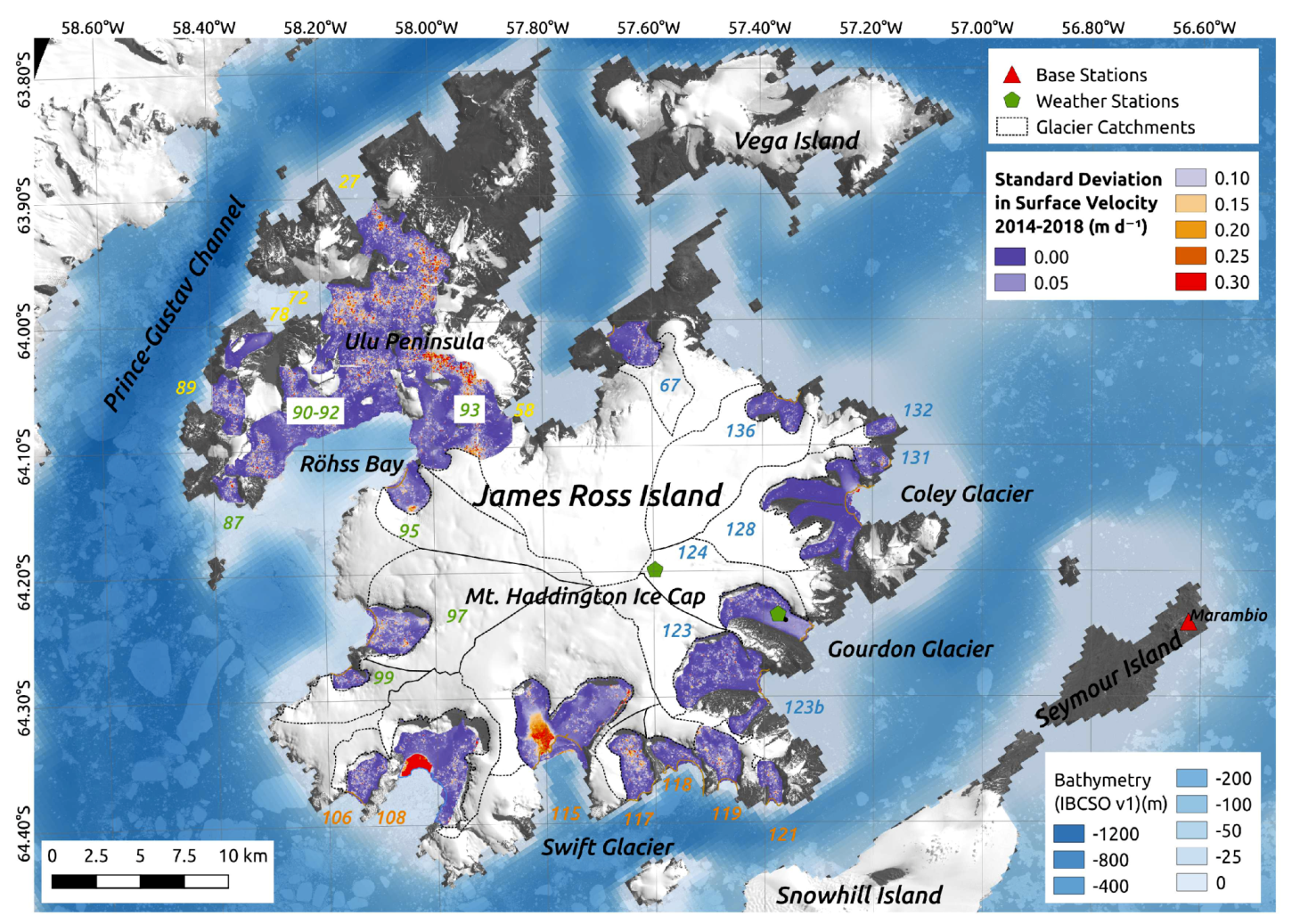
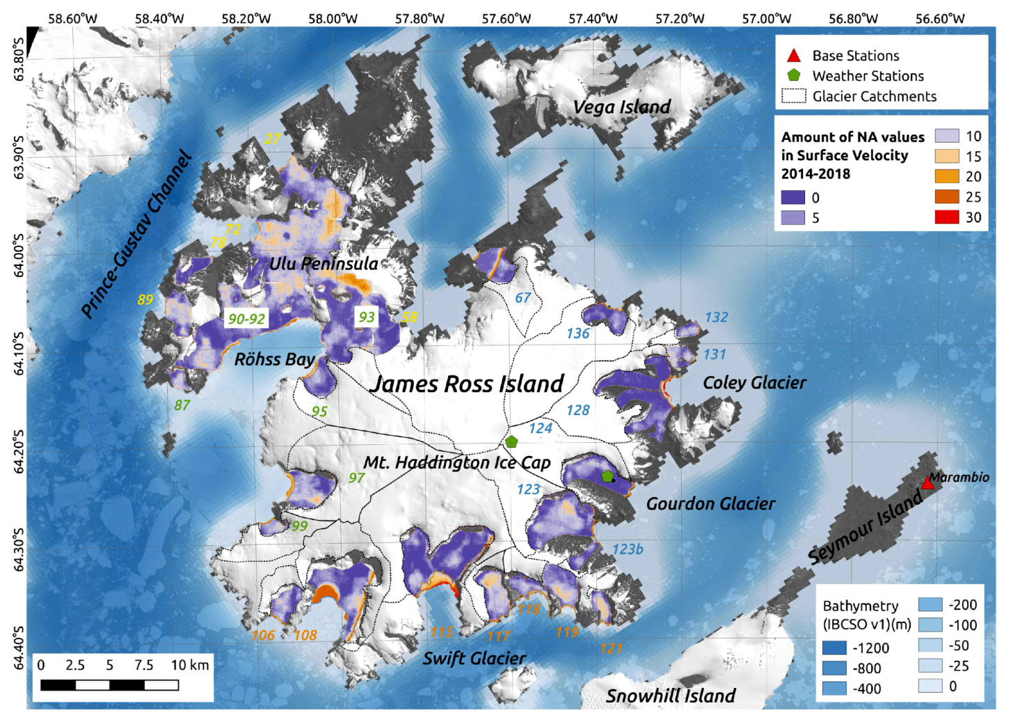
4.1.1. Spatial Variability

The spatially and temporally averaged mean velocity of all evaluated glaciers between 2014 and 2018 is 0 . 077 m d 1 (Table 1). Of course, much higher values occur locally (Figure 2) because the spatial mean is strongly influenced by the slower upper glacier areas. Glaciers flowing into the Röhss Bay are slightly faster with a mean of 0 . 104 m d 1 , whereas glaciers at the north and east coast are slightly slower ( 0 . 055 m d 1 ) than the mean. Glaciers at the south coast have a similar average ( 0 . 080 m d 1 ) as the overall mean, but are strongly affected by the high value of 0 . 178 m d 1 for Swift Glacier.
Glaciers surrounding Röhss Bay, especially the ones at the eastern side (93, 95, and 97), as well as Swift (115) and Tait Glacier (108) show locally higher mean velocities (2014–2018) of about 0 . 5 m d 1 in comparison to the other glaciers on JRI (Table 1). On the eastern side of JRI, only the lower half of Gourdon Glacier (124) and the frontal part of the northern tributary of Coley Glacier (128) reach mean velocities of up to 0 . 5 m d 1 . The temporal-mean speed of all other glaciers mostly remained below 0 . 3 m d 1 during the investigated time frame. The highest velocities with values of up to 0 . 85 m d 1 were found for the west tributary of Swift Glacier. However, other glaciers in the vicinity show no signal of higher velocity, e.g., all the four glaciers at the east side of Swift Glacier (117–121), Hobbs Glacier (123) directly in the south from Gourdon Glacier, and the glaciers in the north from Coley Glacier (131, 132). From the data in Table 2, it can be seen that Swift Glacier has a relatively large accumulation area on the plateau, with a value surpassed only by glaciers at the Röhss Bay and (136).

4.1.2. Temporal Variability
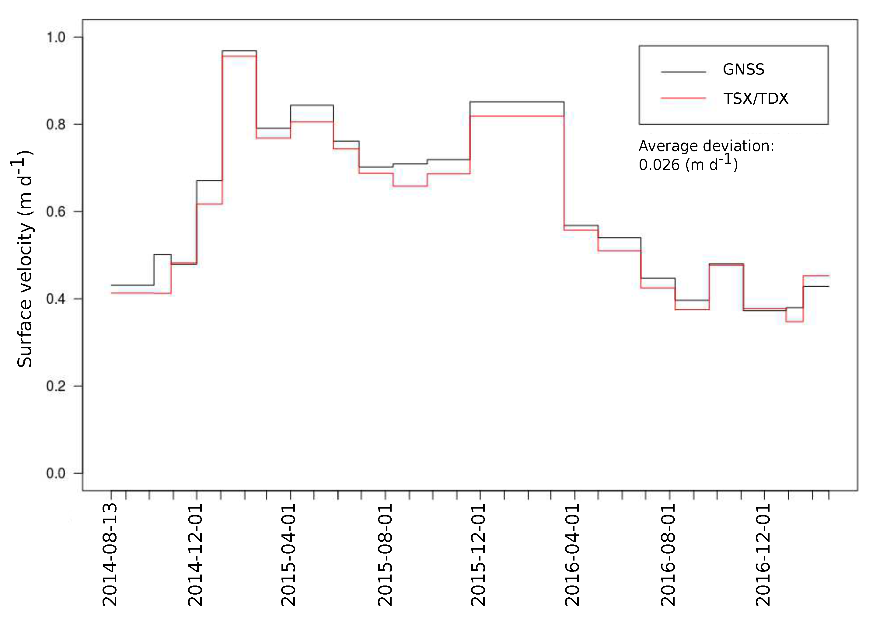
Besides the spatial velocity variation, the temporal variability should also be investigated. Regarding this, Figure A1 shows the temporal standard deviations and Figure A2 shows the coverage of no-data values. A high standard deviation, as in the case of Swift Glacier, Tait Glacier, and parts of the catchment areas in Röhss Bay, can be a sign of considerable temporal velocity variations within the time frame 2014–2018. Since single velocity estimates can be affected by no-data values due to the challenging conditions for the intensity offset tracking method, or area changes at the front, these have to be considered. For example, the higher standard deviation at the frontal part of Tait Glacier can be attributed to area gain at the end of the observing period, leading to velocity measurements for only the last months. In addition, for the glaciers in the Röhss Bay, the higher standard deviations are at locations with a high occurrence of no-data values, in this case due to difficulties in feature tracking. For most other glaciers, the standard deviation is relatively low. Slightly higher values were observed for the parts of Coley and Gourdon Glacier. As these glaciers, along with Swift Glacier, show a large degree of temporal variability, we selected them for the more detailed analysis of area changes (Section 4.2.2). Coley and Gourdon Glacier are located near the weather station at the plateau. This facilitates the validation of modeled meteorological data with the in-situ measurements.

4.1.3. Validation

The surface velocities from satellite data were validated with daily in-situ data from GNSS loggers (August 2014 to February 2017) installed at Gourdon Glacier (Figure 2). The results are shown in Figure 3 where the mean error of 0 . 026 m d 1 is similar to the mean error of 0 . 024 m d 1 (Table A1) estimated with the method from Seehaus et al. [37]. This implies that for slower glaciers the error is no more than half the estimated average velocity.

4.2. Area Changes

For reasons of a clear visualization, Figure 2 shows glacier-retreat areas created by the common-box approach only for three time intervals: The retreat from the maximum extent in 1945–1987 to 1988, the retreat between 1988 and 2008/2009, and the retreat from 2008/2009 until the maximum extent in 2014–2018. Detailed area values (also the occurrence of area losses or gains in the time frame 2014–2018) are presented in Table A3. Due to inconsistent observing dates, we decided to calculate the area retreat before 1987 with regard to the maximum observed extent, even if the time interval available for most of the glaciers is larger than the 20 a from 1988–2008/2009 (Table A3).

4.2.1. General Overview

The estimated annual area change rates suggest a higher retreat rate during 1988–2008/2009 than before (Table 1). Glaciers on the Ulu Peninsula (27, 58, and 72–89) show the smallest increase in area retreat rates ( 0 . 040 km 2 a 1 before 1988 and 0 . 047 km 2 a 1 during 1988–2008/2009), and the glacier at the southern coast (106–121) the highest ( 0 . 113 km 2 a 1 before 1988 and 0 . 215 km 2 a 1 from 1988 to 2008/2009). The biggest area loss was during 1997-2008/2009 at the Röhss Bay. In all four regions (JRI North/East, JRI South, Röhss Bay, and Ulu Peninsula) the annual area loss during 1988–2008/2009 was the highest for the different time intervals, with an overall rate of 1 . 646 km 2 a 1 including Röhss Bay and 0 . 128 km 2 a 1 by excluding Röhss Bay.
No large area loss can be visually observed between 2008/2009 and the maximum extent of 2014–2018 (Figure 2). Considering the detailed area change rates in Table 1, the recession rates of almost all glaciers considerably slowed down from 2008/2009 to 2014 in comparison to during 1988–2008/2009. Some glaciers even gained area during 2014–2018 (e.g., Tait Glacier (108) and Gourdon Glacier (124)), resulting in even a positive area change rate of 0 . 030 km 2 a 1 for JRI South. Area loss from 2014–2018 for glaciers at Röhss Bay and on Ulu Peninsula further slowed down. In contrast, the averaged area loss between 2014 and 2018 at JRI North/East increased to levels similar to the rate between the maximum extent (1945–1987) and 1988.

4.2.2. Detailed Analysis for Selected Glaciers

In the following, area changes are presented in detail for Coley, Gourdon, and Swift Glacier. The outlet area (apparent area in Figure 2) of each time step is added to the catchment area from Davies et al. [15] for a comparison of their overall area. The variability in the area within one year is smaller than the observed area changes before 2009. Therefore, we suggest that the long-term trends of the older measurements are not substantially seasonally biased.
The RMSE between the annual area change from 1988 to 2008/2009 for each of our measured glaciers in comparison to the associated value in Davies et al. [15] is 0 . 19 km 2 a 1 , implying differences in estimates of area change, e.g. in the lateral borders of the common-box for the area calculation.
Considering the detailed analysis of total area values (including catchment) in Figure 4 (blue dots), all three glaciers have suffered a significant area loss in outlet area since the first measurement in 1945/1952. The glacier with the largest area loss is Swift Glacier (Figure 4c), which lost 31 % of its area, followed by 20 % for Coley Glacier (Figure 4a) and 12 % for Gourdon Glacier (Figure 4b). Gourdon Glacier had phases of area gain (e.g., 1964–1974) and even advanced since 2014 to almost the same area as in 2009. However, when evaluating the area change relative to the previous value (grey bars in Figure 4), there is no consistent pattern visible between the three glaciers. Between 1974 and 1979, large ice masses at the terminus of Gourdon Glacier calved off after a period of terminus advance. Swift Glacier lost area during the entire observation period, except 1952–1964, and from 1 March 2014 to 1 March 2016. This is congruent to phases of area gain for Gourdon Glacier, but in contrast Coley Glacier advanced between March and November 2017 and retreated between 1 March 2016 and 1 March 2017.

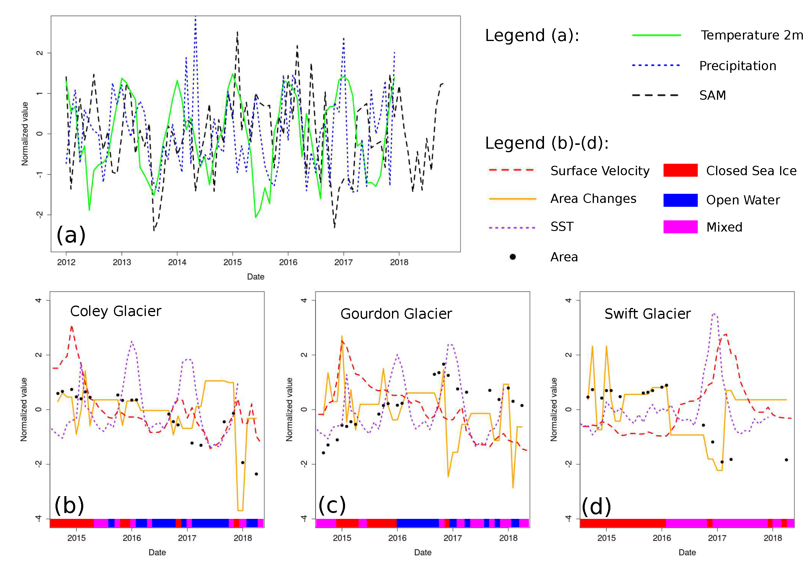
4.3. Potential Forcing Factors of Temporal Velocity Variations

The potential forcing factors of temporal velocity variations were visually evaluated using their normalized values (converted to an arithmetic mean of zero and a standard deviation of 1, Figure 5) for three different glaciers (Coley, Gourdon, and Swift Glacier). Besides the glacier area changes, SSTs and the SAM index, we focused on MAR near-surface air temperature (∼ 2 m above ground) and precipitation on the plateau of JRI. The suitability of these data, especially regarding temporal variability, was validated in Appendix B. In Appendix C, we provide more detailed information on a correlation analysis with different time-lags for all meteorological variables.
The temporal evolution of velocities differ between the three glaciers. Coley (Figure 5b) and Gourdon (Figure 5c) Glacier, at the northeast and east coast of JRI, have one strong peak in surface flow velocity in austral summer 2014/2015. This is followed by a slow deceleration until early summer 2016/2017. Coley Glacier shows two further peaks in the austral summers 2016/2017 and 2017/2018, whereas Gourdon Glacier shows only a slightly speed-up in austral summer 2016/2017. Swift Glacier (Figure 5d) has only one peak in velocity in austral summer 2016/2017. The outlet area of Coley Glacier in the time interval 2014–2018 steadily decreased except for two months in spring 2017. Gourdon Glacier gained area until spring 2016, and slightly lost area afterwards, consistent with the decreasing velocities. Swift Glacier showed a constant area loss from January 2016 to December 2016, with slight gain in area before. At exactly the same time when the area loss was initiated, the velocity of the glacier increased, which indicates an acceleration due to a calving event. However, slightly before the strongest increase in velocity, in the middle of the year 2016, the SSTs abruptly rose. This is in contrast to the SSTs for Coley and Gourdon Glacier, where no significant increase from seasonal variability is visible.
When considering temperature and precipitation at the plateau of JRI, as well as the SAM index (Figure 5a), there is no clear relationship to the observed velocity evolution. Temperature values do not show any change in seasonal variability and precipitation values show only a slight increase in summer 2013/2014 and 2016/2017. The summer 2016/2017 shows higher than average surface velocities for all glaciers. However, a change in velocity or area forced by snowfall in the catchment area is expected to have a considerable time lag. A strong relationship of meteorological parameters with the SAM index observed at other locations at the Antarctic Peninsula [28,31,32], but also for JRI [13], is not visible for the observed glacier surface velocity and area changes.
The sea ice assessment (Figure 5b–d) from Sentinel-1 data reveals a general trend from closed/mixed to mixed/open conditions for Coley and Gourdon Glacier. Moreover, the acceleration phase of Swift Glacier is simultaneous with the change from closed to mixed sea ice conditions.

5. Discussion

5.1. Velocity Analysis

Averaged glacier velocities on JRI during 2014–2018 range from 0.055 m d 1 at the northeast coast of JRI to 0.104 m d 1 at Röhss Bay. However, higher velocities are observed mainly for glaciers in the eastern part of Röhss Bay. In comparison to the other glaciers on JRI, these glaciers (95, 97, and 99) have a larger relative accumulation area on the plateau. For glaciers on the northern side of Röhss Bay and Ulu Peninsula, values could be biased to slower velocities because the catchment areas are included in the calculation of the mean value. Near to the glacier front, some of the glaciers flowing into Röhss Bay reach mean flow speeds of up to 0.5 m d 1 . We were able to apply intensity feature tracking to one scene pair from Phased Array L-Band Synthetic Aperture Radar of the Advanced Land Observing Satellite (ALOS PALSAR) sensor from 26 November 2010 to 11 January 2011. The observed mean surface velocities for the northern Röhss Bay were already very slow ( 0.004 m d 1 ) in summer 2010/2011. Glaciers 93 and 95 showed higher velocities of about 0.2 m d 1 and 0.4 m d 1 . These data indicate that at least for the south-eastern glaciers at the Röhss Bay (95, 97, and 99), velocities did not substantially decreased. However, a maxium velocity value of 0.9 m d 1 in summer 2008/2009 reported by Glasser et al. [14] was not reached.
Considering the monthly velocity data of the three glaciers assessed in depth (Coley, Gourdon, and Swift Glacier), all of them show only a partial seasonal pattern (Figure 5b–d), superimposed with many other effects. The normalized value of their highest peak in velocity exceeded the regular peaks during summer. Osmanoglu et al. [55] reported overall higher velocities in summer than winter at Livingston Island (Figure 1) between 2007 and 2011, with large inter-annual and seasonal variations in surface velocities. At some glaciers on the east side of Livingston Island, seasonal variations were observed [55], but for most of the other glacier basins occasionally increased velocities during winter were possible. Besides an influence from SSTs, this could indicate that periods of surface melting or liquid precipitation occur sporadically during winter at the northern Antarctic Peninsula, which is possibly the result of Föhn events. However, except of Swift Glacier in winter 2016, none of the three selected glaciers on JRI accelerated during winter time (Figure 5b–d). Glacier runoff and the availability of meltwater can play a significant role in controlling glacier velocity. Observations and modeling experiments on the Greenland Ice Sheet reveal an early summer acceleration followed by mid-summer deceleration when an efficient hydrological system evolves analogously to alpine glaciers [56,57]. The observed velocity peaks for Coley, Gourdon, and Swift Glacier occured mostly between December and February. Gourdon Glacier in 2017 and Coley Glacier in 2017 and 2018 suggest a slight slowdown in January, partially supporting the thesis of mid-summer deceleration. However, also a multi-year evolution of the hydrological system could be the reason of the observed peaks in surface velocity.

5.2. Area Changes

The annual area change of glacier calving fronts suggests a slow-down in retreat since the period 1988–2008/2009 from 0.128 km 2 a 1 to 0.093 km 2 a 1 during 2008/2009–2014 and 0.039 km 2 a 1 during 2014–2018. If including the area loss by the Röhss Bay, the retreat rate from 1988–2008/2009 would be even higher ( 1.646 km 2 a 1 ). Especially for the shorter time intervals after 2008/2009, the impact of single glaciers advancing (e.g., Tait Glacier (108)) on the mean values for each region is large. However, observations suggest that most glaciers on JRI are still retreating, with a major proportion of retreating glaciers located on the Röhss Bay.
The spatial pattern of area change between 1988 and 2008/2009, where the highest increase in retreat rate is in the JRI South region, is in contrast to the results from Scambos et al. [8], who observed that the lowest mass loss between 2001 and 2010 was in the southern part. However, the time interval of the measured area change is longer, and glacier elevation change can be independent of any changes in the outlet area.
Area measurements from this study can be compared with those of Davies et al. [15] for the dates 29 February 1988, 1 October 1997, and 3 March 2009 for each of the three glaciers assessed (Figure 4). The differences are normally relative small with values < 2 % , except of Coley Glacier which has a deviation 3.2 % in 1988. A constant deviation suggests that the area calculation is always biased by the same value (e.g., due to different borders at the cliff or at rocky areas beside the tributaries). A stronger deviation for only one time interval suggests either a deviation in the outline areas from Davies et al. [15] or a real change in the accumulation area. This would not be mapped by the processing with fixed polygons, but is very unlikely because the ice cap is relatively stable on the plateau during this time period. The relatively constant deviations between this new dataset and Davies et al. [15] demonstrate that the reported area values are suitable for the analysis of outlet area changes.

5.3. Potential Forcing Factors of Temporal Velocity Variations

Except for Swift Glacier, visual inspection of the peaks in the normalized values of the surface velocity along with the other potential forcings (Figure 5) does not reveal any hints of a clear trigger for acceleration. The impact of oceanic and meteorological factors on any particular glacier can be highly variable and affected by many local factors [58]. These could be the mass flux upstream [59], the geometry of the glacier surface and calving front relative to the sea level [60], the bedrock topography, and the bathymetry of the proglacial fjord [61].
The potential influence from deeper oceanic layers was investigated using data from the IBCSO v1.0 dataset [26] (Figure 2). Reliable multi-beam data exist for deeper areas ∼ 15 km east of Swift Glacier (∼ 500 m b . s . l . (meters below sea level)), the Prince-Gustav-Channel (up to 1000 m b . s . l . ) and the east coast of Ulu Peninsula (∼ 330 m b . s . l . ). At the north-east coast, IBCSO data indicate shallow regions (< 100 m b . s . l . ) between ∼ 2 km and 5 km away from the glacier calving fronts. For the bays directly in front of the outlet glaciers, multi-beam data are available only for Swift Glacier and imply a depth of ∼ 190 m b . s . l . on the former glacier-covered area. The local bathymetry on the other glacier bays can only be assessed from the interpolated data in IBCSO, which report an improbable fixed depth of 10 m b . s . l . near to the fronts of most glaciers.
Glaciers in immediate proximity have likely experienced a similar atmospheric and oceanic forcing. However, the temporal velocity variability as described for Coley, Gourdon and Swift Glacier was not observed for their neighboring glaciers. Thus, we suggest that for relative small outlet glaciers, such as those observed on JRI, the local bathymetry at the glacier calving front strongly controls the impact of the ocean.
Ocean temperatures are suggested to have a high impact on marine-terminating glaciers [17,18,62,63]. Vallot et al. [63] combined the Elmer/Ice ice-flow model and the Helsinki Discrete Element Model (HiDEM) to evaluate the effect of subglacial drainage and mixing with the ocean during the melt season for the Kronebreen tidewater glacier in Svalbard. They observed that undercutting and calving play a key role for glacier retreat. The role of subglacial melt at ocean depths ranging 100–200 m b . s . l . has been investigated in Antarctica for glaciers surrounding George VI Ice Shelf [62], Maguerite Bay [18] and ice shelf retreat along the Antarctic Peninsula [17]. The observed SSTs and the sea ice conditions enabled us to partially assess the influence of oceanic conditions. Except for austral summer 2016/2017 when Swift Glacier accelerated, SSTs at the southern coast of JRI are normally about 0.5 C lower than at the north and east coast. The acceleration of Swift Glacier started shortly after the change from closed to mixed sea ice conditions (Figure 5d), whereas the peak in the SST is delayed and much shorter in the duration. This indicates that the measured NOAA OI SSTs are not generally affected by the sea ice conditions. However, both are supposed to have a strong impact on the surface velocity and the area changes of Swift Glacier.

6. Conclusions

This study reported surface velocities and outlet area changes for JRI from 2014–2018, and evaluated the area changes in a long-term context using calving front positions from previous studies. By considering the main outlet areas, the annual recession rates of the glacier fronts suggest a slow-down since the period 1988–2008/2009 from 1.646 km 2 a 1 to 0.093 km 2 a 1 in 2008/2009–2014 and 0.039 km 2 a 1 in 2014–2018. However, the area loss from 1988 to 2008/2009 is strongly affected by the ice shelf loss in the Röhss Bay, and would be 0.128 km 2 a 1 by excluding it. Slightly higher velocities than the overall average for JRI were observed for the eastern Röhss Bay, Gourdon, and Swift Glacier. Swift Glacier was the only glacier where a strong signal of temporal variability in velocity during 2014–2018 clearly coincides with area loss and an increase in oceanic temperatures. The lack of a clear spatial pattern across multiple glaciers for velocity and area changes, but the sporadic acceleration of some single glaciers, suggests that the bathymetry controls the local impact of oceanic forcing and partially over-modulates the atmospheric influence. Beside information about the distribution and seasonality of sub-glacial volume and drainage, higher resolved oceanic data are necessary to assess the influence of sub-glacial melt at the glacier front. With this knowledge, a better evaluation of the super-position of oceanic and atmospheric influences on velocity and area changes would be possible.

Author Contributions

Conceptualization, S.L. and M.H.B.; Formal analysis, S.L., P.F. and C.K.; Funding acquisition, M.H.B.; Investigation, S.L., S.M., T.-C.S. and M.H.B.; Methodology, S.L., P.F., C.K. and T.-C.S.; Project administration, S.M. and M.H.B.; Software, S.L. and T.-C.S.; Supervision, M.H.B.; Visualization, S.L.; Writing—original draft, S.L.; and Writing—review and editing, S.L., P.F., C.K., S.M., T.-C.S. and M.H.B.

Funding

This study was funded by the Deutsche Forschungsgemeinschaft (DFG) in the framework of the priority programme “Antarctic Research with comparative investigations in Arctic ice areas” by grants to M.H.B. (BR 2105/9-1 and BR 2105/13-1). We would like to thank the HGF Alliance “Remote Sensing of Earth System Dynamics” for additional support. TS was financially supported by the DLR/BMWi grant GEKKO (50EE1544). Costs covered by our Argentinian partner were funded by the project from ’Balance de masa y dinámica de glaciares en la Península Antártica’ from Instituto Antártico Argentino. Access to satellite data was kindly provided by various space agencies, e.g., under ESA AO 4032, DLR TerraSAR-X Background Mission Antarctic Peninsula and Ice Shelves, TSX AO LAN0013, TanDEM-X Mission TDX AO XTI_GLAC0264, ASF, and GLIMS as well as NASA and USGS.

Conflicts of Interest

The authors declare no conflict of interest.

Abbreviations

The following abbreviations are used in this manuscript:
ADDAntarctic Digital Database
a.s.l.above sea level
AWSAutomatic Weather Station
b.s.l.below sea level
ELAEquilibrium Line Altitude
GLIMSGlobal Land Ice Measurements from Space
GNSSGlobal Navigation Satellite System
IBCSOInternational Bathymetric Chart of the Southern Ocean
JRIJames Ross Island
MARModèle Atmosphérique Régional
MERRA-2Modern-Era Retrospective Analysis for Research and Applications version 2
RMSEroot-mean-square error
SAMSouthern Annular Mode
SARSynthetic Aperture Radar
SCARScientific Committee on Antarctic Research
SSTSea Surface Temperature
TDXTanDEM-X
TSXTerraSAR-X
w.e.water equivalent

Appendix A. Detailed Information of Applied Satellite Scenes for Intensity Feature Tracking and Area Calculations

Figure A1. Temporal standard deviation of the surface velocity estimations 2014–2018 derived from intensity feature tracking. Glacier catchments are from Davies et al. [15]. Background: Landsat-8 (20 February 2017) ©U.S. Geological Survey and bathymetric data [26].
Geosciences 09 00374 g0a1
Figure A2. Amount of no-data (NA) values per pixel in the surface velocity estimations 2014–2018 derived from intensity feature tracking. The overall amount of TSX/TDX scenes in Table A1 is 31 for the east side (glaciers 115–136, southern part of 67) and 27 for the west side (glaciers 27–108, northern part of 67) of JRI. Glacier catchments are from Davies et al. [15]. Background: Landsat-8 (20 February 2017) ©U.S. Geological Survey and bathymetric data [26].
Geosciences 09 00374 g0a2
Table A1. Satellite scenes with associated error estimates used as slave and master image in intensity feature tracking.
Sensor Scene 1PathDate Scene 1Abs. Orbit Scene 1Date Scene 2Abs. Orbit Scene 2Time Step (days) σ v T (m d 1 ) σ v C (m d 1 ) σ v SUM (m d 1 )
TSX0140-0142014-08-1322,9892014-10-0723,824550.0050.0090.010
TDX0140-0142014-10-0723,8242014-10-2924,158220.0110.0140.018
TDX0140-0142014-10-2924,1582014-12-0124,659330.0080.0210.022
TSX0140-0142014-12-0124,6592015-01-0341,890330.0080.0100.013
TSX0140-0142015-01-0341,8902015-02-1642,558440.0060.0220.023
TSX0140-0142015-02-1642,5582015-04-0143,226440.0060.0030.007
TSX0140-0142015-04-0143,2262015-05-2644,061550.0050.0070.008
TSX0140-0142015-05-2644,0612015-06-2844,562330.0080.0100.013
TSX0140-0142015-06-2844,5622015-08-1145,230440.0060.0100.011
TSX0140-0142015-08-1145,2302015-09-2445,898440.0060.0070.009
TSX0140-0142015-09-2445,8982015-11-1846,733550.0050.0180.018
TSX0140-0142015-11-1846,7332016-03-1848,5701210.0020.0180.018
TSX0140-0142016-03-1848,5702016-05-0149,238440.0060.0090.011
TSX0140-0142016-05-0149,2382016-06-2550,073550.0050.0060.007
TSX0140-0142016-06-2550,0732016-08-0850,741440.0060.0060.008
TDX0140-0142016-08-0850,7412016-09-2134,679440.0060.0090.010
TDX0140-0142016-09-2134,6792016-11-0435,347440.0060.1050.105
TDX0140-0142016-11-0435,3472016-12-2936,182550.0050.1660.166
TDX0140-0142016-12-2936,1822017-01-2036,516220.0110.0590.061
TDX0140-0142017-01-2036,5162017-02-2237,017330.0080.0200.022
TDX0140-0142017-02-2237,0172017-03-2737,518330.0080.0070.010
TDX0140-0142017-03-2737,5182017-05-1038,186440.0060.0080.010
TDX0140-0142017-05-1038,1862017-06-0138,520220.0110.0110.016
TDX0140-0142017-06-0138,5202017-07-1539,188440.0060.0070.009
TDX0140-0142017-07-1539,1882017-08-2839,856440.0060.0110.012
TSX0140-0142017-08-2839,8562017-10-1157,254440.0060.0130.014
TSX0140-0142017-10-1157,2542017-11-2457,922440.0060.0720.072
TSX0140-0142017-11-2457,9222018-01-0758,590440.0060.0070.009
TSX0140-0142018-01-0758,5902018-02-2059,258440.0060.0060.009
TSX0140-0142018-02-2059,2582018-04-0559,926440.0060.0530.053
TSX0140-0142018-04-0559,9262018-05-1960,594440.0060.0080.010
TSX0034-0042014-11-1324,3862014-12-0541,450220.0110.0310.033
TSX0034-0042014-12-0541,4502015-04-2743,6211430.0020.0030.004
TSX0034-0042015-04-2743,6212015-06-1044,289440.0060.0080.010
TSX0034-0042015-06-1044,2892015-07-2444,957440.0060.0070.009
TSX0034-0042015-07-2444,9572015-09-1745,792550.0050.0050.007
TSX0034-0042015-09-1745,7922015-11-1146,627550.0050.0140.015
TSX0034-0042015-11-1146,6272016-02-2948,2971100.0020.0130.014
TDX0034-0042016-02-2948,2972016-04-1332,235440.0060.0140.015
TSX0034-0042016-04-1332,2352016-06-0749,800550.0050.0030.005
TDX0034-0042016-06-0749,8002016-09-0334,406880.0030.0080.008
TDX0034-0042016-09-0334,4062016-10-1735,074440.0060.0180.019
TDX0034-0042016-10-1735,0742016-11-3035,742440.0060.0110.013
TDX0034-0042016-11-3035,7422016-12-2236,076220.0110.0420.043
TDX0034-0042016-12-2236,0762017-01-1336,410220.0110.0680.069
TDX0034-0042017-01-1336,4102017-02-1536,911330.0080.0390.039
TDX0034-0042017-02-1536,9112017-03-2037,412330.0080.0090.012
TDX0034-0042017-03-2037,4122017-04-2237,913330.0080.0080.011
TDX0034-0042017-04-2237,9132017-05-2538,414330.0080.0110.013
TDX0034-0042017-05-2538,4142017-07-0839,082440.0060.0040.007
TDX0034-0042017-07-0839,0822017-09-1240,084660.0040.0170.018
TSX0034-0042017-09-1240,0842017-10-0457,148220.0110.0220.025
TSX0034-0042017-10-0457,1482017-11-1757,816440.0060.0540.054
TSX0034-0042017-11-1757,8162017-12-3158,484440.0060.0480.048
TSX0034-0042017-12-3158,4842018-02-1359,152440.0060.0360.037
TSX0034-0042018-02-1359,1522018-03-2959,820440.0060.0170.018
TSX0034-0042018-03-2959,8202018-05-1260,488440.0060.0780.078
TSX0034-0042018-05-1260,4882018-06-2561,156440.0060.0060.008
Mean 0.0060.0230.024
Table A2. Satellite scenes used for the delineation of glacier fronts.
SensorDateWRS PathWRS Row
Landsat 82014-01-11215105
Landsat 82014-01-18216105
Landsat 82014-03-16215105
Landsat 82014-03-23216105
Landsat 82014-04-01215105
Landsat 82014-09-24215105
Landsat 82014-10-03214105
Landsat 82014-11-02216105
Landsat 82014-12-04216105
Landsat 82015-01-30215105
Landsat 82015-02-06216105
Landsat 82015-03-28214105
Landsat 82015-04-20215105
Landsat 82015-09-11215105
Landsat 82015-09-18216105
Landsat 82015-10-20216105
Landsat 82015-11-05216105
Landsat 82015-11-30215105
Landsat 82016-01-17215105
Landsat 82016-02-02215105
Landsat 82016-02-18215105
Landsat 82016-09-22214105
Landsat 82016-10-06216105
Landsat 82016-11-25214105
Landsat 82016-12-09216105
Landsat 82016-12-11214106
Landsat 82016-12-16217105
Landsat 82016-12-25216106
Landsat 82017-02-04215105
Landsat 82017-02-20215105
Landsat 82017-03-08215105
Landsat 82017-04-25215105
Landsat 82017-08-22216105
Landsat 82017-09-23216105
Landsat 82017-09-25214105
Landsat 82017-09-30217105
Landsat 82017-10-09216105
Landsat 82017-10-27214105
Landsat 82017-11-10216105
Landsat 82017-11-28214105
Landsat 82017-12-03217105
Landsat 82018-01-06215105
Landsat 82018-01-15214105
Landsat 82018-02-07215105
Landsat 82018-04-03216105
Table A3. Calculated area values (including catchment areas from Davies et al. [15]) by the common-box approach. Fronts (before 2014) are from Davies et al. and SCAR ADD [15,16]. For 2014 and 2018, they are derived from newly digitized Landsat-8 scenes and are displayed by taking the average of January to April.
GLIMS IDArea (km 2 ) 1945-02-01Area (km 2 ) 1952-08-01Area (km 2 ) 1964-09-26Area (km 2 ) 1974-06-21Area (km 2 ) 1979-01-12Area (km 2 ) 1988-02-29Area (km 2 ) 1997-10-01Area (km 2 ) 2000-02-21Area (km 2 ) 2008-03-09Area (km 2 ) 2009-03-03Area (km 2 ) 2014-03-01Area (km 2 ) 2018-03-01
James Ross Island North/East
G302417E64049S (67)37.7 37.26 36.3136.1436
G302479E64128S (136)112.42 111.39 110.35110.29110.38
G302771E64094S (132)8.6 8.25 7.587.477.36
G302783E64108S (131)6.79 6.6 6.216.216.19
G302579E64173S (128) 104.58 101.61 95.5295.5493.91
G302503E64208S (124) 78.73 76.28 74.6974.2474.63
G302436E64248S (123), G302547E64322S (123b) 93.1 91.85 89.2989.6189.41
James Ross Island South
G302603E64361S (121) 8.417.91 6.476.316.24
G302508E64342S (119) 15.56 15.07 13.9113.7813.66
G302425E64325S (118) 21.3 19.98 18.8618.9918.62
G302333E64350S (117) 29.51 28.84 26.6126.4826.66
G302228E64270S (115) 69.44 60.9 49.6748.645.83
G302012E64324S (108) 110.93 104.66 92.5689.3393.48
G301861E64353S (106) 25.88 25.32 22.9423.0422.88
Röhss Bay
(99) 38.52 38.0138.1
G302028E64232S (97) 125.73 125.23123.98
G302020E64160S (95) 73.8 72.1672.02
Röhss Bay East (93) 66.73 65.7765.56
Röhss Bay North (90–92) 72.19 69.6268.55
G301629E64129S (87) 5.82 5.81 5.375.32
Röhss Bay Ice Shelf 330.88221.93 0
Ulu Peninsula
G301636E64062S (89)14.26 13.76 12.3412.3312.23
G301659E64016S (78) 7.24 77.337.82
G301912E63989S (72)74.51 70.8 70.3869.6269.07
G301946E63935S (27)33.01 30.54 28.6328.3628.12
G302104E64073S (58) 21.9 21.71 20.4820.41
Table A4. Satellite scenes used for the classification of sea ice conditions.
SensorDateTimeOrbit CycleRel. OrbitAbs. Orbit
SENTINEL-1A2014-10-0812:19:3517402735
SENTINEL-1A2014-10-0812:26:4217402735
SENTINEL-1A2014-11-0111:06:1232383085
SENTINEL-1A2014-11-0110:54:3932383085
SENTINEL-1A2014-12-0710:34:4335383610
SENTINEL-1A2014-12-0710:58:2535383610
SENTINEL-1A2015-01-1210:03:3638384135
SENTINEL-1A2015-01-1210:05:1238384135
SENTINEL-1A2015-02-0510:27:4440384485
SENTINEL-1A2015-02-0510:27:4740384485
SENTINEL-1A2015-03-2510:24:1044385185
SENTINEL-1A2015-03-2510:31:0044385185
SENTINEL-1A2015-04-1810:28:4246385535
SENTINEL-1A2015-04-1810:22:3746385535
SENTINEL-1A2015-05-1416:59:5548385885
SENTINEL-1A2015-05-1417:06:4348385885
SENTINEL-1A2015-06-1710:03:2551386410
SENTINEL-1A2015-06-1712:35:4351386410
SENTINEL-1A2015-07-1111:19:2353386760
SENTINEL-1A2015-07-1111:20:0053386760
SENTINEL-1A2015-08-1609:46:2256387285
SENTINEL-1A2015-08-1609:41:2656387285
SENTINEL-1A2015-09-0909:39:1658387635
SENTINEL-1A2015-09-0909:39:5958387635
SENTINEL-1A2015-10-1509:38:1361388160
SENTINEL-1A2015-10-1509:39:4861388160
SENTINEL-1A2015-11-2009:58:3564388685
SENTINEL-1A2015-11-2009:55:3964388685
SENTINEL-1A2015-12-1409:56:3266389035
SENTINEL-1A2016-01-1915:26:5669389560
SENTINEL-1A2016-02-1210:17:2271389910
SENTINEL-1A2016-03-0711:10:42733810,260
SENTINEL-1A2016-04-1209:55:33763810,785
SENTINEL-1A2016-05-1809:32:52793811,310
SENTINEL-1A2016-06-1109:39:44813811,660
SENTINEL-1A2016-07-0509:37:35833812,010
SENTINEL-1A2016-08-1009:37:17863812,535
SENTINEL-1A2016-07-0309:36:30883812,885
SENTINEL-1A2016-10-0909:33:33913813,410
SENTINEL-1A2016-11-0209:41:38933813,760
SENTINEL-1A2016-12-0809:36:20963814,285
SENTINEL-1A2017-01-0109:41:46983814,635
SENTINEL-1A2017-02-0609:37:261013815,160
SENTINEL-1A2017-03-0209:40:511033815,510
SENTINEL-1A2017-04-0710:34:431063816,035
SENTINEL-1A2017-05-0109:36:101083816,385
SENTINEL-1A2017-06-0609:36:211113816,910
SENTINEL-1A2017-07-1209:38:491143817,435
SENTINEL-1A2017-08-0509:42:561163817,785
SENTINEL-1A2017-07-2209:46:091203818,485
SENTINEL-1A2017-10-1609:44:491223818,835
SENTINEL-1A2017-11-0909:35:211243819,185
SENTINEL-1A2017-12-0309:45:221263819,535
SENTINEL-1B2018-01-0209:46:3558388989
SENTINEL-1B2018-02-0714:01:2161389514
SENTINEL-1B2018-03-0309:46:5463389864
SENTINEL-1B2018-04-0809:33:07663810,389
SENTINEL-1B2018-05-1409:35:21693810,914

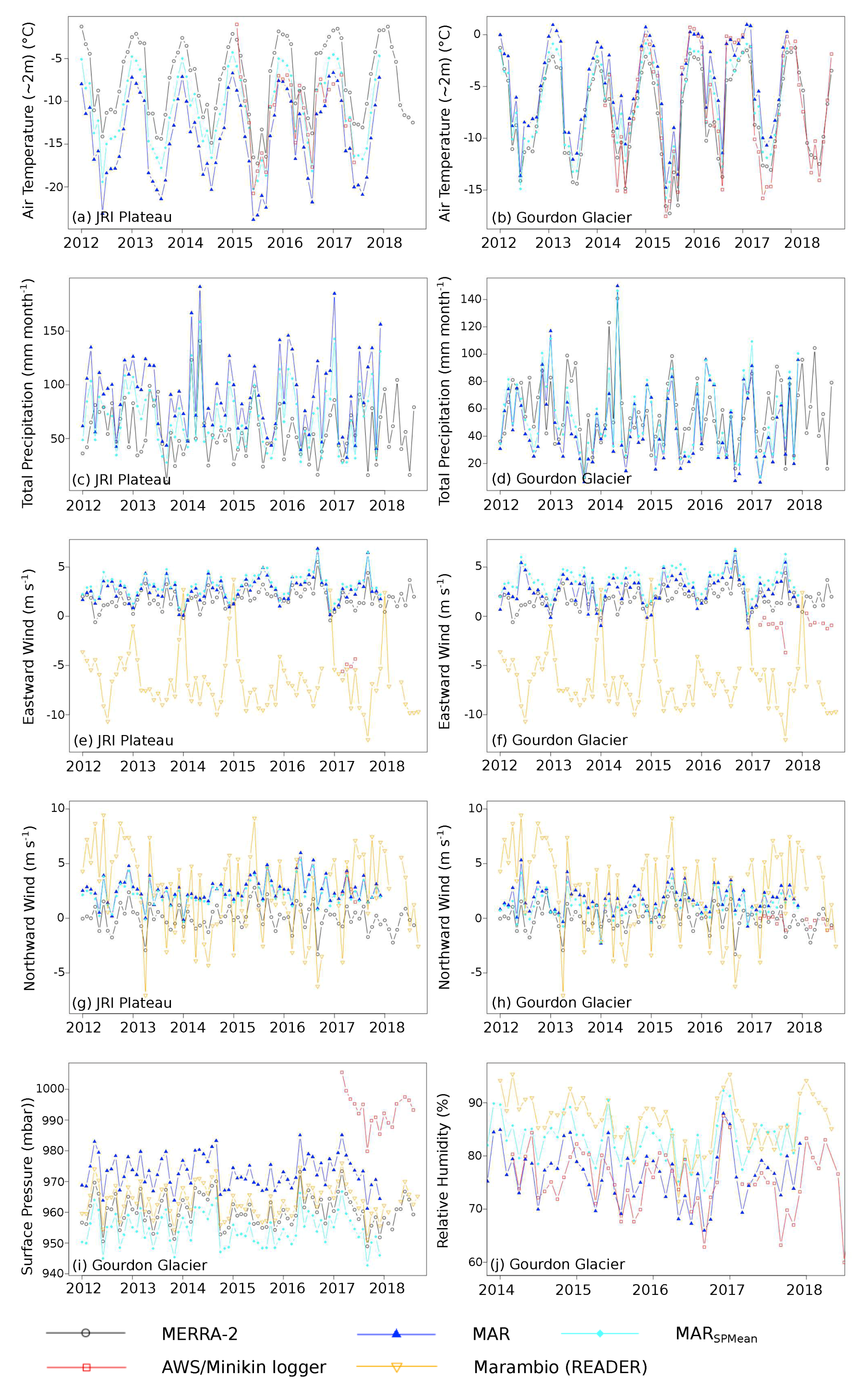
Appendix B. Comparison of Meteorological Data

This section compares model and reanalysis meteorological data with in-situ measurements on Gourdon Glacier (elevation of ∼ 100 m a . s . l . ), the plateau of the island (∼ 1400 m a . s . l . ) and data from Marambio station on Seymour Island (∼ 200 m a . s . l . , available via the READER project) (all locations are in Figure 2). The comparison should evaluate which of the modeled and reanalysis data really reflect the climate conditions on JRI and are suitable for the correlation analysis (Appendix C). When calculating root-mean-square errors (RMSE) between different variables, only the overlapping time frame for all data is considered. The associated time frames for each meteorological variable with in-situ data from the two automatic weather stations (AWS) (Campbell Scientific, Inc) and the two Minikin loggers (EMS Brno) are listed in Table A5.
Table A5. Time spans of in-situ, model, and reanalysis data for the comparison of different meteorological variables.
Climate VariableMERRA-2MARAWS/MinikinMarambioSSTSAM
Temperature 2 m PlateauJanuary 2012– August 2018January 2012– December 2017March 2015– June 2017
Temperature 2 m GourdonJanuary 2012– November 2018January 2012– December 2017March 2014– November 2018
Precipitation PlateauJanuary 2012– August 2018January 2012– December 2017
Precipitation GourdonJanuary 2012– August 2018January 2012– December 2017
Northward Wind Plateau 2 mJanuary 2012– August 2018January 2012– December 2017March 2017– June 2017January 2012– September 2018
Eastward Wind Plateau 2 mJanuary 2012– August 2018January 2012– December 2017March 2017– June 2017January 2012 September 2018
Northward Wind Gourdon 2 mJanuary 2012– August 2018January 2012– December 2017March 2017– August 2018January 2012– September 2018
Eastward Wind Gourdon 2 mJanuary 2012– August 2018January 2012– December 2017March 2017– August 2018January 2012– September 2018
Relative Humidity Gourdon 2 m January 2012– December 2017March 2014– August 2018January 2014– May 2018
Surface Pressure GourdonJanuary 2012– August 2018January 2012– December 2017March 2017– August 2018January 2012– September 2018
Sea Surface Temperature January 2012– December 2017
Southern Annular Mode January 2012– September 2018
In addition to the model data from MAR, long-term reanalyzed climate data from the Modern-Era Retrospective Analysis for Research and Applications version 2 (MERRA-2) dataset produced by the Goddard Earth Observation System-5 (GEOS-5) atmospheric general circulation model (AGCM) [64,65] were included in the comparison. The data are freely accessible at a resolution of 0 . 50 × 0 . 65 , and have been widely used all over the world. Nevertheless, local small-scale features such as the outlet glaciers on JRI with, e.g., a width smaller than 2 km , are not resolved by MERRA-2. We used the nearest grid point to the in-situ data, located at 64 S , 57 . 5 W (Figure 2).
At the plateau (Figure A3a), near-surface air temperature values at 2 m above ground from the spatially averaged MAR SpMean (Section 3.3) agree best with our in-situ measurements with a RMSE of 1.64 C in contrast to 4.05 C for MERRA-2 and 3.53 C for MAR. At Gourdon Glacier (Figure A3b), it is more difficult to assess the best climate dataset. During austral summer half-year (October–March), MAR has a lower RMSE than MAR SpMean ( 1.15 C vs. 1.61 C ). The RMSE between April and September is very high for MAR ( 3.60 C ), whereas the difference between summer and winter for MERRA-2 is lower ( 2.19 C and 2.13 C ). This implicates that for higher temperatures during summer time at low elevations such as the outlet of Gourdon Glacier, MAR data without averaging agree very well with the in-situ data, but they do not reproduce the cold values during winter.
Figure A3. Comparison of monthly means for different meteorological variables from model, reanalysis, and in-situ data: (a,b) surface temperature; (c,d) precipitation; (e,f) eastward wind; (g,h) northward wind; (i) surface pressure; and (j) relative humidity. Data from MAR and the AWS/Minikin loggers were split between JRI Plateau and the Gourdon Glacier, whereas data from MERRA-2 and Marambio are constant. No corrections for elevation were applied. All locations are in Figure 2.
Geosciences 09 00374 g0a3
The other meteorological data often show higher deviations between model and in-situ data than temperature values (Figure A3c–j). Especially the interpretation of wind vector data (Figure A3e–h) is difficult, because in-situ data from the AWS and from the adjacent Marambio station also disagree. In the case of the measurements on the Gourdon Glacier, this could be at least partially explained by different wind conditions in the shadow of the high cliff wall. Nevertheless, data from the plateau are also difficult to explain because the AWS data for northward wind (Figure A3g) fit better to the MAR data (RMSE: 0.77 m s 1 ) than to the Marambio data (RMSE: 4.23 m s 1 ). Instead, for eastward wind (Figure A3e), the AWS data fit better to the Marambio data with a RMSE of 2.24 m s 1 in contrast to 7.42 m s 1 for the MAR and 6.57 m s 1 for the MERRA-2 data. Modeled relative surface pressure (Figure A3i) and humidity data (Figure A3j) show a constant offset due to our low elevation location at the Gourdon glacier. For both, the RMSEs during winter and summer time are almost the same (e.g., 20.92 mbar for MAR and 39.69 mbar for MAR SpMean during April–September, and 20.67 mbar for MAR and 39.18 mbar for MAR SpMean during October–March). Therefore, the seasonal variability is similar and both were tested as input in the correlation analysis. For precipitation (Figure A3c,d), where no field data are available, the MAR and MERRA-2 data on the plateau strongly differ with a RMSE of 45.10 mm month 1 and a high variability.
The analysis of meteorological data from different sources (model, reanalysis, and in situ data) revealed that higher resolution models such as MAR are able to partially reflect the local conditions at the small and narrow outlet glaciers on JRI. Seasonal variability is correctly reflected for near-surface air temperature, surface pressure, and partially also relative humidity, implying a suitability of all these variables for correlation analysis. Of course, surface pressure and relative humidity are more susceptible to a bias due to the location of in-situ data, especially when a difference in elevation occurs. We resigned any correction of elevation bias in Figure A3 to underline this impact. In the case of correlation analysis, data only have to show the same temporal variability to ensure comparability. In addition to visual inspection in Figure A3, we tested this for near-surface air temperature, surface pressure, and relative humidity by calculating the correlation between in-situ data and MAR (Table A6). Especially near-surface air temperature and surface pressure show high correlation with Kendall’s tau from values of 0.80 . Wind datasets are too short to reveal reasonable correlation factors. Additionally, in the case of wind, it has to be investigated why both MAR and MERRA-2 reflect in-situ northward, but not the eastward wind situations on both the plateau and the Gourdon Glacier. The difference between data from Gourdon Glacier and Marambio station implies uncertainties resulting from local conditions.
Table A6. Correlations (Kendall’s tau and Kendall’s p) between in-situ measurements, MAR, and MAR SpMean . Details to correlation tests applying the “Kendall” approach can be found in Appendix C.
Climate VariablesIn-Situ with MARIn-Situ with MAR SpMean MAR with MAR SpMean
Kendall’s TauKendall’s pKendall’s TauKendall’s pKendall’s TauKendall’s p
Temperature 2 m Plateau0.80 3 . 8 × 10 12 0.80 2 . 3 × 10 12 0.98 8 . 8 × 10 16
Temperature 2 m Gourdon0.80 4 . 4 × 10 16 0.80 4 . 4 × 10 16 0.96 4 . 4 × 10 16
Relative Humidity Gourdon 2 m0.390.0001140.360.0004670.91 4 . 4 × 10 16
Surface Pressure Gourdon1.00 5 . 5 × 10 7 0.96 5 . 5 × 10 6 0.96 5 . 5 × 10 6

Appendix C. Correlation Analysis

The surface velocity measurements were correlated with area changes and meteorological variables by calculating “Kendall’s” tau and the associated p-value. “Kendall’s” tau is a non-parametric measure of the strength of the relationship between two ordinal level variables [66]. A small p-value indicates a more significant relationship. Correlation tests applying the “Kendall” approach are also useful for small datasets, and in comparison to the “Pearson” method also a monotonic relationship in the data is sufficient [67]. Gaps in the monthly area measurements were filled by linear interpolation. Therefore, a positive bias in the correlation with area cannot be excluded and we decided not to use them as a primary estimator such as velocity. First, the correlation test was done without any time-lag. Afterwards, temporal shifts of up to 18 months were introduced for the second variable, in order to account for possible time-lagged correlations with the surface velocity. For example, a positive time-lag of one month means that the velocity values were correlated with each value of the month before of the second variable. Additionally, a threshold of minimum 30 remaining entries in the dataset was applied. However, the latter produced a break in correlation only for area data where such a long time-lag is not probable [68].
All Kendall’s tau and p values for every time-lag and every meteorological variable applied are in Table A7Table A11. It has to be considered that the datasets have 30–50 entries, depending on the time-lag. Due to the relatively small amount of data, the absolute values in the correlation coefficient have a higher variability. For Coley Glacier, no significant high tau-values were observed between velocity and area changes as well as the SAM for time-lag zero. Only a very weak correlation of about 0.25–0.27 exists for surface air and ocean temperatures. The SAM in the same year does not show any correlation. When applying time-lags and searching for the maximum absolute correlation, we found a weak correlation of 0.23 for a time lag of seven months in the case of the area changes and −0.24 for a time lag of 13 months in the case of the SAM. SSTs and atmospheric temperatures show a slightly stronger negative correlation of −0.41 and −0.39 when applying a time-lag of six months. For Gourdon Glacier, there is only a week correlation of 0.23–0.24 with area changes and the SAM applying no time-lag, and no significant higher values with temperatures at the sea surface and both weather stations. Correlation with area changes is highest (0.34) applying a time-lag of six months. A weak correlation with SSTs (−0.22) can be observed for a seven months time-lag, which probably only reflects the half-yearly seasonal temperature pattern. The temporal overlay of velocity increase with the peak in SSTs for Swift Glacier is not visible in a stronger correlation. No correlation was found with a zero time-lag and only a weak correlation of 0.22 for a time lag of 6–8 months. However, we found a weak correlation with the SAM (0.26) and a correlation coefficient of −0.41 with the area changes. By applying a time lag of two-to-three months, it can be increased to −0.29 for the SAM and −0.51 for the area changes. The latter one is the highest absolute correlation coefficient, which was observed for the three glaciers and combinations of all variables. However, the correlation analysis of SSTs and velocity data does not show a clear relationship as for the other meteorological variables. This could be due to superimposed effects from different atmospheric and oceanic changes. Correlation failed probably also due to the different time scales the changes are happening. For example, a change in area due to a calving event can be linked to a specific date or at least a month but the induced velocity change will prolong for several months. In addition, other variables such as atmospheric or oceanic changes can have a much shorter duration than the resulting velocity changes. This hypothesis is supported by a longer temporal auto-correlation of velocity data. The velocity data show significant correlation in a time interval of three months for Coley Glacier, five to nine months for Gourdon Glacier, and six to seven months for Swift Glacier. Besides the half-yearly occurrence of higher tau-values after some months in the case of seasonal-driven data such as temperature, no conspicuous temporal autocorrelation were detected.
Table A7. Kendall’s tau and Kendall’s p output from the correlation analysis of monthly surface velocity values with the stated variable. Correlation values stated in the text are in bold.
Time-LagKendall’s TauKendall’s pKendall’s TauKendall’s pKendall’s TauKendall’s p
Coley GlacierGourdon GlacierSwift Glacier
Area changes
0−0.120.270.230.03−0.410.00
1−0.010.960.210.05−0.470.00
20.001.000.210.06−0.500.00
30.060.570.190.08−0.510.00
40.160.150.260.02−0.440.00
50.200.070.320.00−0.340.00
60.220.050.340.00−0.330.00
70.230.050.300.01−0.300.01
80.170.150.260.03−0.190.10
90.110.350.170.15−0.110.34
100.060.600.130.29−0.100.41
110.001.000.120.31−0.050.69
120.070.580.140.250.040.74
130.060.650.070.590.160.21
140.110.400.000.970.300.02
150.150.25−0.010.930.370.01
Air Temperature 2m Plateau
00.270.010.100.350.060.57
10.150.160.110.300.080.45
20.000.970.040.690.120.27
3−0.160.13−0.010.940.100.35
4−0.310.00−0.060.550.100.36
5−0.350.00−0.130.190.130.22
6−0.390.00−0.160.110.160.11
7−0.360.00−0.190.060.190.07
8−0.180.08−0.200.050.170.09
9−0.010.95−0.150.130.160.12
100.120.24−0.120.260.130.21
110.230.02−0.090.360.160.13
120.250.02−0.050.660.060.57
130.210.04−0.010.950.020.84
140.110.29−0.010.950.000.96
15−0.050.63−0.050.62−0.010.95
16−0.230.03−0.070.47−0.030.77
17−0.330.00−0.160.130.010.91
Sea Surface Temperature (SST)
00.250.020.160.14−0.010.92
10.120.270.140.200.020.88
2−0.050.650.060.570.040.74
3−0.200.050.000.990.060.55
4−0.310.00−0.100.340.130.21
5−0.370.00−0.160.110.180.08
6−0.410.00−0.200.050.220.03
7−0.300.00−0.220.030.220.03
8−0.110.28−0.200.050.220.03
90.050.64−0.170.090.170.10
100.180.08−0.150.140.180.08
110.270.01−0.090.400.170.10
120.350.00−0.040.690.130.21
130.330.00−0.010.910.180.08
140.240.02−0.020.820.190.07
150.050.62−0.030.740.210.04
16−0.090.38−0.070.510.160.12
17−0.220.03−0.140.180.170.10
Table A8. Kendall’s tau and Kendall’s p output from the correlation analysis of monthly surface velocity values with the stated variable. Correlation values stated in the text are in bold.
Time-LagKendall’s TauKendall’s pKendall’s TauKendall’s pKendall’s TauKendall’s p
Coley GlacierGourdon GlacierSwift Glacier
Southern Annular Mode
00.050.620.240.02−0.260.01
10.070.480.230.03−0.260.01
20.030.810.110.26−0.290.00
3−0.090.380.070.50−0.230.03
4−0.040.670.070.49−0.220.04
50.030.770.080.42−0.200.05
6−0.010.890.140.16−0.250.02
70.060.580.160.11−0.130.21
80.110.260.180.08−0.130.21
90.080.440.130.20−0.140.17
100.030.780.070.490.070.50
11−0.040.700.070.510.050.62
12−0.140.170.001.000.100.31
13−0.240.020.030.760.070.48
14−0.190.070.010.890.140.16
15−0.180.080.030.740.120.26
16−0.200.05−0.030.750.260.01
17−0.160.11−0.100.330.180.08
Precipitation Plateau
00.080.47−0.060.56−0.090.41
10.060.580.020.85−0.050.63
20.070.520.150.15−0.100.33
30.200.060.150.17−0.020.86
4−0.020.850.110.30−0.010.94
5−0.050.620.070.500.080.45
60.120.240.040.680.040.70
7−0.010.900.050.660.030.81
80.000.98−0.040.71−0.020.82
90.080.440.000.98−0.010.92
100.080.460.040.720.030.75
110.200.050.060.580.000.98
120.120.240.180.080.030.78
130.140.180.200.060.010.92
140.010.910.210.040.000.98
15−0.040.680.100.310.010.89
16−0.120.240.000.98−0.030.78
17−0.100.33−0.070.500.001.00
Northward Wind Plateau 2 m
0−0.040.740.040.70−0.070.50
1−0.050.660.030.79−0.030.75
2−0.060.540.010.93−0.030.75
3−0.050.61−0.010.900.040.67
40.020.870.100.31−0.090.37
50.030.750.040.66−0.040.71
6−0.030.740.010.930.050.65
70.000.98−0.040.710.000.97
8−0.050.630.020.81−0.020.86
9−0.100.32−0.020.840.070.51
10−0.170.10−0.080.450.090.39
11−0.280.01−0.080.430.080.44
12−0.240.02−0.140.170.230.03
13−0.230.02−0.170.100.170.10
14−0.250.01−0.130.210.220.03
15−0.170.10−0.140.180.180.08
16−0.060.58−0.200.050.160.11
17−0.160.12−0.160.120.150.14
Table A9. Kendall’s tau and Kendall’s p output from the correlation analysis of monthly surface velocity values with the stated variable. Correlation values stated in the text are in bold.
Time-LagKendall’s TauKendall’s pKendall’s TauKendall’s pKendall’s TauKendall’s p
Coley GlacierGourdon GlacierSwift Glacier
Eastward Wind Plateau 2 m
0−0.220.050.020.88−0.100.35
1−0.070.49−0.030.75−0.070.52
20.010.93−0.030.790.010.91
30.080.470.030.770.070.48
40.200.050.010.950.020.81
50.190.060.080.46−0.020.84
60.200.050.080.44−0.060.58
70.190.060.090.40−0.030.75
80.030.740.030.770.040.69
9−0.130.220.010.920.060.57
10−0.260.01−0.050.650.070.51
11−0.380.00−0.050.620.060.53
12−0.390.00−0.100.330.100.35
13−0.360.00−0.180.080.170.10
14−0.280.01−0.180.080.200.05
15−0.110.28−0.160.130.200.05
16−0.010.93−0.110.280.170.09
170.070.50−0.160.130.130.21
Precipitation Gourdon
00.100.38−0.040.70−0.090.42
10.010.960.010.94−0.040.74
2−0.050.660.140.18−0.100.35
30.090.400.100.33−0.030.78
4−0.080.450.110.29−0.040.70
5−0.080.460.050.640.070.49
60.100.320.020.840.070.47
70.020.840.010.930.010.92
80.060.53−0.010.93−0.050.60
90.140.16−0.010.92−0.030.78
100.130.200.070.470.010.95
110.230.020.100.34−0.030.78
120.140.180.210.040.010.92
130.130.220.200.050.010.92
140.001.000.210.04−0.020.83
15−0.080.440.060.540.000.97
16−0.180.09−0.060.54−0.020.86
17−0.200.05−0.080.420.020.83
Air Temperature 2m Gourdon
00.210.050.140.180.080.47
10.080.480.110.300.080.45
2−0.050.650.030.750.140.19
3−0.200.06−0.040.740.120.25
4−0.360.00−0.090.360.130.22
5−0.400.00−0.160.120.130.19
6−0.400.00−0.180.070.170.10
7−0.340.00−0.190.060.190.06
8−0.150.14−0.200.050.210.04
9−0.010.92−0.150.140.200.05
100.110.29−0.140.180.170.10
110.190.07−0.120.230.210.04
120.170.09−0.090.370.100.34
130.120.25−0.080.460.050.60
140.030.81−0.080.450.040.67
15−0.110.30−0.120.230.060.56
16−0.270.01−0.120.250.040.67
17−0.380.00−0.210.040.080.42
Table A10. Kendall’s tau and Kendall’s p output from the correlation analysis of monthly surface velocity values with the stated variable. Correlation values stated in the text are in bold.
Time-LagKendall’s TauKendall’s pKendall’s TauKendall’s pKendall’s TauKendall’s p
Coley GlacierGourdon GlacierSwift Glacier
Northward Wind Gourdon 2 m
0−0.120.27−0.070.54−0.070.53
1−0.060.57−0.050.64−0.020.82
2−0.040.720.000.97−0.040.71
30.040.720.000.990.050.64
40.070.510.060.55−0.100.35
50.090.360.030.73−0.070.49
60.080.450.000.98−0.040.69
70.090.39−0.060.56−0.070.48
8−0.070.490.010.92−0.080.43
9−0.100.31−0.020.83−0.010.94
10−0.150.140.000.980.020.85
11−0.240.020.030.810.020.83
12−0.170.09−0.020.810.140.18
13−0.150.14−0.080.460.110.29
14−0.160.12−0.080.430.150.15
150.000.99−0.060.580.130.21
160.090.37−0.090.380.080.44
170.030.74−0.040.670.100.33
Eastward Wind Gourdon 2 m
0−0.250.02−0.040.72−0.100.38
1−0.100.37−0.080.48−0.080.44
20.010.95−0.040.71−0.040.71
30.120.250.020.880.040.72
40.240.020.030.760.010.92
50.270.010.070.48−0.010.90
60.290.000.090.38−0.080.45
70.240.020.100.35−0.040.66
80.100.350.080.450.010.92
9−0.070.480.060.590.000.98
10−0.200.050.020.850.040.69
11−0.330.000.010.890.020.85
12−0.360.00−0.020.870.040.66
13−0.330.00−0.100.310.090.40
14−0.270.01−0.140.180.130.21
15−0.130.21−0.140.180.140.18
16−0.010.95−0.080.450.110.28
170.130.21−0.100.340.070.47
Rel. Humidity Gourdon 2 m
00.170.12−0.090.410.010.93
10.100.350.000.990.030.80
20.090.390.100.34−0.080.43
30.160.130.070.50−0.080.43
40.000.980.110.30−0.160.12
5−0.010.940.050.65−0.090.37
60.080.410.080.45−0.060.54
7−0.050.620.000.98−0.120.23
8−0.010.93−0.010.90−0.190.06
90.060.580.000.96−0.190.06
100.140.170.050.61−0.110.26
110.230.020.090.39−0.190.06
120.250.010.190.06−0.120.24
130.300.000.270.01−0.150.14
140.260.010.270.01−0.170.10
150.220.030.220.03−0.220.03
160.190.060.150.13−0.220.03
170.110.290.170.09−0.160.12
Table A11. Kendall’s tau and Kendall’s p output from the correlation analysis of monthly surface velocity values with the stated variable. Correlation values stated in the text are in bold.
Time-LagKendall’s TauKendall’s pKendall’s TauKendall’s pKendall’s TauKendall’s p
Coley GlacierGourdon GlacierSwift Glacier
Surface Pressure Gourdon
0−0.110.33−0.050.670.270.01
1−0.100.36−0.140.200.280.01
2−0.080.44−0.200.060.320.00
3−0.090.41−0.220.040.220.04
40.030.79−0.150.150.260.01
50.100.34−0.080.430.210.04
60.030.77−0.090.400.250.01
70.070.51−0.070.480.150.15
80.160.11−0.010.920.080.46
90.140.180.020.830.080.43
100.070.480.000.980.001.00
110.010.92−0.060.54−0.010.89
12−0.060.59−0.100.34−0.130.21
13−0.080.42−0.090.39−0.150.13
14−0.090.38−0.110.30−0.150.13
15−0.140.16−0.140.16−0.140.17
16−0.090.40−0.090.38−0.200.05
17−0.070.48−0.030.74−0.220.03

Appendix D. Processing of Outlet Areas with the Common-Box Approach

Figure A4. (a) Manual digitization of the fixed reference outlet polygon (red area) using the side boundaries from Davies et al. [15] (red line) and the visible brim of the cliff in a Landsat-8 scene from 20 February 2017. (b) If the original glacier calving front lines (black and blue) from the existing inventories [15,16] do not cut the reference polygon, slight modifications (yellow) are made to create reasonable glacier outlines. (c) Example for the resulting calving front for the year 1988 (blue area). (d) Resulting overall outlet area (blue) for the year 1988. Background: Landsat-8 (20 February 2017) ©U.S. Geological Survey.
Geosciences 09 00374 g0a4

References

  1. Turner, J.; Colwell, S.R.; Marshall, G.J.; Lachlan-Cope, T.A.; Carleton, A.M.; Jones, P.D.; Lagun, V.; Reid, P.A.; Iagovkina, S. Antarctic climate change during the last 50 years. Int. J. Climatol. 2005, 25, 279–294. [Google Scholar] [CrossRef]
  2. Vaughan, D.G.; Marshall, G.J.; Connolley, W.M.; Parkinson, C.; Mulvaney, R.; Hodgson, D.A.; King, J.C.; Pudsey, C.J.; Turner, J. Recent rapid regional climate warming on the Antarctic Peninsula. Clim. Chang. 2003, 60, 243–274. [Google Scholar] [CrossRef]
  3. Oliva, M.; Navarro, F.; Hrbáček, F.; Hernández, A.; Nývlt, D.; Pereira, P.; Ruiz-Fernández, J.; Trigo, R. Recent regional climate cooling on the Antarctic Peninsula and associated impacts on the cryosphere. Sci. Total Environ. 2016. [Google Scholar] [CrossRef] [PubMed]
  4. Skvarca, P. Fast recession of the northern Larsen Ice Shelf monitored by space images. Ann. Glaciol. 1993, 17, 317–321. [Google Scholar] [CrossRef] [Green Version]
  5. Skvarca, P.; Rott, H.; Nagler, T. Satellite imagery, a base line for glacier variation study on James Ross Island, Antarctica. Ann. Glaciol. 1995, 21, 291–296. [Google Scholar] [CrossRef] [Green Version]
  6. Rott, H.; Skvarca, P.; Nagler, T. Rapid Collapse of Northern Larsen Ice Shelf, Antarctica. Science 1996, 271, 788–792. [Google Scholar] [CrossRef]
  7. Rott, H.; Rack, W.; Nagler, T.; Skvarca, P. Climatically induced retreat and collapse of northern Larsen Ice Shelf, Antarctic Peninsula. Ann. Glaciol. 1998, 27, 86–92. [Google Scholar] [CrossRef] [Green Version]
  8. Scambos, T.A.; Berthier, E.; Haran, T.; Shuman, C.A.; Cook, A.J.; Ligtenberg, S.R.M.; Bohlander, J. Detailed ice loss pattern in the northern Antarctic Peninsula: widespread decline driven by ice front retreats. Cryosphere 2014, 8, 2135–2145. [Google Scholar] [CrossRef] [Green Version]
  9. Turner, J.; Lu, H.; White, I.; King, J.C.; Phillips, T.; Hosking, J.S.; Bracegirdle, T.J.; Marshall, G.J.; Mulvaney, R.; Deb, P. Absence of 21st century warming on Antarctic Peninsula consistent with natural variability. Nature 2016, 535, 411–415. [Google Scholar] [CrossRef] [Green Version]
  10. Engel, Z.; Láska, K.; Nývlt, D.; Stachoň, Z. Surface mass balance of small glaciers on James Ross Island, north-eastern Antarctic Peninsula, during 2009–2015. J. Glaciol. 2018, 64, 349–361. [Google Scholar] [CrossRef]
  11. WGMS. Global Glacier Change Bulletin No. 2 (2014–2015); Zemp, M., Nussbaumer, S.U., Gärtner-Roer, I., Huber, J., Machguth, H., Paul, F., Hoelzle, M., Eds.; ICSU(WDS)/IUGG(IACS)/UNEP/UNESCO/WMO, World Glacier Monitoring Service: Zurich, Switzerland, 2017. [Google Scholar] [CrossRef]
  12. WGMS. Submitted values for Global Glacier Change Bulletin Version 3. 2019. Available online: https://wgms.ch/latest-glacier-mass-balance-data/ (accessed on 1 July 2019).
  13. Abram, N.J.; Mulvaney, R.; Arrowsmith, C. Environmental signals in a highly resolved ice core from James Ross Island, Antarctica. J. Geophys. Res. Atmos. 2011, 116. [Google Scholar] [CrossRef] [Green Version]
  14. Glasser, N.F.; Scambos, T.A.; Bohlander, J.; Truffer, M.; Pettit, E.; Davies, B.J. From ice-shelf tributary to tidewater glacier: continued rapid recession, acceleration and thinning of Röhss Glacier following the 1995 collapse of the Prince Gustav Ice Shelf, Antarctic Peninsula. J. Glaciol. 2011, 57, 397–406. [Google Scholar] [CrossRef]
  15. Davies, B.J.; Carrivick, J.L.; Glasser, N.F.; Hambrey, M.J.; Smellie, J.L. Variable glacier response to atmospheric warming, northern Antarctic Peninsula, 1988–2009. Cryosphere 2012, 6, 1031–1048. [Google Scholar] [CrossRef]
  16. SCAR. Antarctic Digital Database. 2018. Available online: https://www.add.scar.org/ (accessed on 22 November 2018).
  17. Cook, A.J.; Holland, P.R.; Meredith, M.P.; Murray, T.; Luckman, A.; Vaughan, D.G. Ocean forcing of glacier retreat in the western Antarctic Peninsula. Science 2016, 353, 283–286. [Google Scholar] [CrossRef] [PubMed] [Green Version]
  18. Walker, C.C.; Gardner, A.S. Rapid drawdown of Antarctica’s Wordie Ice Shelf glaciers in response to ENSO/Southern Annular Mode-driven warming in the Southern Ocean. Earth Planet. Sci. Lett. 2017, 476, 100–110. [Google Scholar] [CrossRef]
  19. Friedl, P.; Seehaus, T.C.; Wendt, A.; Braun, M.H.; Höppner, K. Recent dynamic changes on Fleming Glacier after the disintegration of Wordie Ice Shelf, Antarctic Peninsula. Cryosphere 2018, 12, 1347–1365. [Google Scholar] [CrossRef] [Green Version]
  20. Rabassa, J.; Skvarca, P.; Bertani, L.; Mazzoni, E. Glacier Inventory of James Ross and Vega Islands, Antarctic Peninsula. Ann. Glaciol. 1982, 3, 260–264. [Google Scholar] [CrossRef] [Green Version]
  21. Ferrigno, J.G.; Cook, A.J.; Foley, K.M.; Williams, R.S., Jr.; Swithinbank, C.; Fox, A.J.; Thomson, J.W.; Sievers, J. Coastal-Change and Glaciological Map of the Trinity Peninsula Area and South Shetland Islands, Antarctica: 1843-2001: Chapter A in Coastal-Change and Glaciological Maps of Antarctica; USGS Numbered Series 2600-A; U.S. Geological Survey: Reston, VA, USA, 2006.
  22. Arigony-Neto, J.; Skvarca, P.; Marinsek, S.; Braun, M.; Humbert, A.; Junior, C.W.M.; Jaña, R. Monitoring Glacier Changes on the Antarctic Peninsula. In Global Land Ice Measurements from Space; Kargel, J.S., Leonard, G.J., Bishop, M.P., Kääb, A., Raup, B.H., Eds.; Springer: Berlin/Heidelberg, Germany, 2014; pp. 717–741. [Google Scholar]
  23. Smellie, J.L.; Johnson, J.S.; McIntosh, W.C.; Esser, R.; Gudmundsson, M.T.; Hambrey, M.J.; van Wyk de Vries, B. Six million years of glacial history recorded in volcanic lithofacies of the James Ross Island Volcanic Group, Antarctic Peninsula. Palaeogeogr. Palaeoclimatol. Palaeoecol. 2008, 260, 122–148. [Google Scholar] [CrossRef]
  24. Jiskoot, H.; Curran, C.J.; Tessler, D.L.; Shenton, L.R. Changes in Clemenceau Icefield and Chaba Group glaciers, Canada, related to hypsometry, tributary detachment, length–slope and area–aspect relations. Ann. Glaciol. 2009, 50, 133–143. [Google Scholar] [CrossRef]
  25. Davies, B.J.; Golledge, N.R.; Glasser, N.F.; Carrivick, J.L.; Ligtenberg, S.R.M.; Barrand, N.E.; van den Broeke, M.R.; Hambrey, M.J.; Smellie, J.L. Modelled glacier response to centennial temperature and precipitation trends on the Antarctic Peninsula. Nat. Clim. Chang. 2014, 4, 993–998. [Google Scholar] [CrossRef] [Green Version]
  26. Arndt, J.E.; Schenke, H.W.; Jakobsson, M.; Nitsche, F.O.; Buys, G.; Goleby, B.; Rebesco, M.; Bohoyo, F.; Hong, J.K.; Black, J.; et al. The International Bathymetric Chart of the Southern Ocean Version 1.0—A new bathymetric compilation covering circum-Antarctic waters. Geophys. Res. Lett. 2013, 40, 1–7. [Google Scholar] [CrossRef]
  27. Morris, E.M.; Vaughan, D.G. Spatial and Temporal Variation of Surface Temperature on the Antarctic Peninsula And The Limit of Viability of Ice Shelves. In Antarctic Peninsula Climate Variability: Historical and Paleoenvironmental Perspectives; American Geophysical Union (AGU): Washington, DC, USA, 2013; pp. 61–68. [Google Scholar]
  28. Marshall, G.J.; Thompson, D.W.J. The signatures of large-scale patterns of atmospheric variability in Antarctic surface temperatures. J. Geophys. Res. Atmos. 2016, 121, 3276–3289. [Google Scholar] [CrossRef]
  29. Cape, M.R.; Vernet, M.; Skvarca, P.; Marinsek, S.; Scambos, T.; Domack, E. Foehn winds link climate-driven warming to ice shelf evolution in Antarctica. J. Geophys. Res. Atmos. 2015, 120. [Google Scholar] [CrossRef]
  30. Van Den Broeke, M.R.; Van Lipzig, N.P.M. Response of Wintertime Antarctic Temperatures to the Antarctic Oscillation: Results of a Regional Climate Model. In Antarctic Peninsula Climate Variability: Historical and Paleoenvironmental Perspectives; American Geophysical Union (AGU): Washington, DC, USA, 2003; pp. 43–58. [Google Scholar] [CrossRef]
  31. Thompson, D.W.J.; Solomon, S. Interpretation of recent Southern Hemisphere climate change. Science 2002, 296, 895–899. [Google Scholar] [CrossRef] [PubMed]
  32. Marshall, G.J.; Thompson, D.W.J.; van den Broeke, M.R. The Signature of Southern Hemisphere Atmospheric Circulation Patterns in Antarctic Precipitation. Geophys. Res. Lett. 2017, 44, 11580–11589. [Google Scholar] [CrossRef] [PubMed]
  33. Marshall, G.J.; Orr, A.; Turner, J. A Predominant Reversal in the Relationship between the SAM and East Antarctic Temperatures during the Twenty-First Century. J. Clim. 2013, 26, 5196–5204. [Google Scholar] [CrossRef] [Green Version]
  34. Moffat, C.; Meredith, M. Shelf–ocean exchange and hydrography west of the Antarctic Peninsula: A review. Philos. Trans. R. Soc. A 2018, 376, 20170164. [Google Scholar] [CrossRef]
  35. Strozzi, T.; Luckman, A.; Murray, T.; Wegmuller, U.; Werner, C.L. Glacier motion estimation using SAR offset-tracking procedures. IEEE Trans. Geosci. Remote Sens. 2002, 40, 2384–2391. [Google Scholar] [CrossRef] [Green Version]
  36. Burgess, E.W.; Forster, R.R.; Larsen, C.F.; Braun, M. Surge dynamics on Bering Glacier, Alaska, in 2008–2011. Cryosphere 2012, 6, 1251–1262. [Google Scholar] [CrossRef]
  37. Seehaus, T.; Cook, A.J.; Silva, A.B.; Braun, M. Changes in glacier dynamics in the northern Antarctic Peninsula since 1985. Cryosphere 2018, 12, 577–594. [Google Scholar] [CrossRef] [Green Version]
  38. Seehaus, T.; Marinsek, S.; Helm, V.; Skvarca, P.; Braun, M. Changes in ice dynamics, elevation and mass discharge of Dinsmoor–Bombardier–Edgeworth glacier system, Antarctic Peninsula. Earth Planet. Sci. Lett. 2015, 427, 125–135. [Google Scholar] [CrossRef]
  39. Moon, T.; Joughin, I. Changes in ice front position on Greenland’s outlet glaciers from 1992 to 2007. J. Geophys. Res. Earth Surf. 2008, 113. [Google Scholar] [CrossRef]
  40. Vijay, S.; Khan, S.A.; Kusk, A.; Solgaard, A.M.; Moon, T.; Bjørk, A.A. Resolving Seasonal Ice Velocity of 45 Greenlandic Glaciers With Very High Temporal Details. Geophys. Res. Lett. 2019. [Google Scholar] [CrossRef]
  41. Cook, A.J.; Vaughan, D.G.; Luckman, A.J.; Murray, T. A new Antarctic Peninsula glacier basin inventory and observed area changes since the 1940s. Antarct. Sci. 2014, 26, 614–624. [Google Scholar] [CrossRef] [Green Version]
  42. De Ridder, K.; Gallée, H. Land Surface-Induced Regional Climate Change in Southern Israel. J. Appl. Meteor. 1998, 37, 1470–1485. [Google Scholar] [CrossRef]
  43. Brun, E.; David, P.; Sudul, M.; Brunot, G. A numerical model to simulate snow cover stratigraphy for operational avalanche forecasting. J. Glaciol. 1992, 38, 13–22. [Google Scholar] [CrossRef]
  44. Gallée, H.; Schayes, G. Development of a Three-Dimensional Meso-Gamma Primitive Equation Model: Katabatic Winds Simulation in the Area of Terra Nova Bay, Antarctica. Mon. Weather Rev. 1994, 122, 671–685. [Google Scholar] [CrossRef]
  45. Lang, C.; Fettweis, X.; Erpicum, M. Future climate and surface mass balance of Svalbard glaciers in an RCP8.5 climate scenario: A study with the regional climate model MAR forced by MIROC5. Cryosphere 2015, 9, 945–956. [Google Scholar] [CrossRef]
  46. Gallée, H.; Trouvilliez, A.; Agosta, C.; Genthon, C.; Favier, V.; Naaim-Bouvet, F. Transport of Snow by the Wind: A Comparison Between Observations in Adélie Land, Antarctica, and Simulations Made with the Regional Climate Model MAR. Bound.-Layer Meteor. 2013, 146, 133–147. [Google Scholar] [CrossRef]
  47. Amory, C.; Trouvilliez, A.; Gallée, H.; Favier, V.; Naaim-Bouvet, F.; Genthon, C.; Agosta, C.; Piard, L.; Bellot, H. Comparison between observed and simulated aeolian snow mass fluxes in Adélie Land, East Antarctica. Cryosphere 2015, 9, 1373–1383. [Google Scholar] [CrossRef]
  48. Fettweis, X.; Box, J.E.; Agosta, C.; Amory, C.; Kittel, C.; Lang, C.; As, D.V.; Machguth, H.; Gallée, H. Reconstructions of the 1900-2015 Greenland ice sheet surface mass balance using the regional climate MAR model. Cryosphere 2017, 11, 1015–1033. [Google Scholar] [CrossRef]
  49. Kittel, C.; Amory, C.; Agosta, C.; Delhasse, A.; Doutreloup, S.; Huot, P.V.; Wyard, C.; Fichefet, T.; Fettweis, X. Sensitivity of the current Antarctic surface mass balance to sea surface conditions using MAR. Cryosphere 2018, 12, 3827–3839. [Google Scholar] [CrossRef] [Green Version]
  50. Agosta, C.; Amory, C.; Kittel, C.; Orsi, A.; Favier, V.; Gallée, H.; van den Broeke, M.R.; Lenaerts, J.T.M.; van Wessem, J.M.; van de Berg, W.J.; et al. Estimation of the Antarctic surface mass balance using the regional climate model MAR (1979–2015) and identification of dominant processes. Cryosphere 2019, 13, 281–296. [Google Scholar] [CrossRef]
  51. Datta, R.T.; Tedesco, M.; Agosta, C.; Fettweis, X.; Kuipers Munneke, P.; van den Broeke, M.R. Melting over the northeast Antarctic Peninsula (1999–2009): Evaluation of a high-resolution regional climate model. Cryosphere 2018, 12, 2901–2922. [Google Scholar] [CrossRef]
  52. Marshall, G.J. An Observation-Based Southern Hemisphere Annular Mode Index. 2018. Available online: https://legacy.bas.ac.uk/met/gjma/sam.html (accessed on 7 March 2019).
  53. NOAA/OAR/ESRL. PSD NOAA OI SST V2, Boulder, Colorado, USA. 2018. Available online: https://www.esrl.noaa.gov/psd/ (accessed on 31 January 2019).
  54. Muckenhuber, S.; Sandven, S. Open-source sea ice drift algorithm for Sentinel-1 SAR imagery using a combination of feature tracking and pattern matching. Cryosphere 2017, 11, 1835–1850. [Google Scholar] [CrossRef] [Green Version]
  55. Osmanoglu, B.; Navarro, F.J.; Hock, R.; Braun, M.; Corcuera, M.I. Surface velocity and mass balance of Livingston Island ice cap, Antarctica. Cryosphere 2014, 8, 1807–1823. [Google Scholar] [CrossRef] [Green Version]
  56. Moon, T.; Joughin, I.; Smith, B.; van den Broeke, M.R.; van de Berg, W.J.; Noël, B.; Usher, M. Distinct patterns of seasonal Greenland glacier velocity. Geophys. Res. Lett. 2014, 41, 7209–7216. [Google Scholar] [CrossRef] [PubMed] [Green Version]
  57. Koziol, C.P.; Arnold, N. Modelling seasonal meltwater forcing of the velocity of land-terminating margins of the Greenland Ice Sheet. Cryosphere 2018, 12, 971–991. [Google Scholar] [CrossRef] [Green Version]
  58. Moon, T.; Joughin, I.; Smith, B.; Howat, I. 21st-Century Evolution of Greenland Outlet Glacier Velocities. Science 2012, 336, 576–578. [Google Scholar] [CrossRef] [Green Version]
  59. Post, A.; O’Neel, S.; Motyka, R.J.; Streveler, G. A complex relationship between calving glaciers and climate. Eos Trans. Am. Geophys. Union 2011, 92, 305–306. [Google Scholar] [CrossRef] [Green Version]
  60. Mercenier, R.; Lüthi, M.P.; Vieli, A. Calving relation for tidewater glaciers based on detailed stress field analysis. Cryosphere Discuss. 2017, 2017, 1–33. [Google Scholar] [CrossRef] [Green Version]
  61. Nick, F.M.; Vieli, A.; Howat, I.M.; Joughin, I. Large-scale changes in Greenland outlet glacier dynamics triggered at the terminus. Nat. Geosci. 2009, 2, 110–114. [Google Scholar] [CrossRef]
  62. Hogg, A.E.; Gudmundsson, G.H. Impacts of the Larsen-C Ice Shelf calving event. Nat. Clim. Chang. 2017, 7, 540–542. [Google Scholar] [CrossRef]
  63. Vallot, D.; Åström, J.; Zwinger, T.; Pettersson, R.; Everett, A.; Benn, D.I.; Luckman, A.; van Pelt, W.J.J.; Nick, F.; Kohler, J. Effects of undercutting and sliding on calving: A global approach applied to Kronebreen, Svalbard. Cryosphere 2018, 12, 609–625. [Google Scholar] [CrossRef]
  64. Molod, A.; Takacs, L.; Suarez, M.; Bacmeister, J. Development of the GEOS-5 atmospheric general circulation model: Evolution from MERRA to MERRA2. Geosci. Model Dev. 2015, 8, 1339–1356. [Google Scholar] [CrossRef]
  65. Gelaro, R.; McCarty, W.; Suárez, M.J.; Todling, R.; Molod, A.; Takacs, L.; Randles, C.A.; Darmenov, A.; Bosilovich, M.G.; Reichle, R.; et al. The Modern-Era Retrospective Analysis for Research and Applications, Version 2 (MERRA-2). J. Clim. 2017, 30, 5419–5454. [Google Scholar] [CrossRef]
  66. Puka, L. Kendall’s Tau. In International Encyclopedia of Statistical Science; Lovric, M., Ed.; Springer: Berlin/Heidelberg, Germany, 2011; pp. 713–715. [Google Scholar]
  67. Hennemuth, B.; Bender, S.; Bülow, K.; Dreier, N.; Keup-Thiel, E.; Krüger, O.; Mudersbach, C.; Radermacher, C.; Schoetter, R. Statistical Methods for the Analysis of Simulated and Observed Climate Data: Applied in Projects and Institutions Dealing with Climate Change Impact and Adaptation; CSC Report 13; Climate Service Center: Hamburg, Germany, January 2013. [Google Scholar]
  68. Walter, J.I.; Box, J.E.; Tulaczyk, S.; Brodsky, E.E.; Howat, I.M.; Ahn, Y.; Brown, A. Oceanic mechanical forcing of a marine-terminating Greenland glacier. Ann. Glaciol. 2012, 53, 181–192. [Google Scholar] [CrossRef] [Green Version]
Figure 1. (a) Map of the location of James Ross Island east of the northern Antarctic Peninsula, the adjacent islands, research stations and ocean regions mentioned in the text. (b) Overview map. Background: ©OpenStreetMap contributors (https://www.openstreetmap.org/copyright).
Geosciences 09 00374 g001
Figure 2. Map of James Ross Island, showing mean surface velocities, selected area changes and the location of in-situ Global Navigation Satellite System (GNSS) measurements. The colored numbers are the local IDs used by Davies et al. [15] and can be related to the adjacent GLIMS-IDs with color-coding for the different regions in Table 1. Glacier catchments are from Davies et al. [15]. The atmospheric model grid cell centers from MAR and MERRA-2 are shown as red dots. Background: Landsat-8 (20 February 2017) ©U.S. Geological Survey and bathymetric data [26].
Geosciences 09 00374 g002
Figure 3. Time series of surface velocities at the outlet of Gourdon Glacier from intensity feature tracking (TSX/TDX scenes) and in-situ GNSS measurements.
Geosciences 09 00374 g003
Figure 4. Absolute areas ( km 2 , blue dots) and area change rates ( km 2 a 1 , grey bars) in comparison to the previous measurement for: (a) Coley Glacier; (b) Gourdon; and (c) Swift Glacier. Area changes before 2014 are based on fronts from existing inventories [15,16], new area measurements from 2014 onwards are displayed two times per year by taking the average of January to April and September to December. Area values from Davies et al. [15] for the years 1988, 1997, and 2009 are plotted as blue diamonds.
Geosciences 09 00374 g004
Figure 5. (a) Normalized value of surface air temperature (green), precipitation (blue), and the Southern Annular Mode (SAM) (black) between 2012 and 2018. (bd) Normalized values of surface velocity (red), area (black), area changes (to the previous month in km 2 , orange) and Sea Surface Temperature (SST) (purple) for: (b) Coley Glacier; (c) Gourdon Glacier; and (d) Swift Glacier. Monthly area changes were calculated from temporally interpolated area data where no Landsat scenes (Table A2) were available. The classification into sea ice conditions was done using one Sentinel-1 GRDH scene per month (Table A4).
Geosciences 09 00374 g005
Table 1. Mean surface velocities (2014–2018) and area change rates for a range of time periods for all glaciers shown in Figure 2.
GLIMS ID (ID in Davies et al. 2012)Velocity Mean (md 1 )Area Change Rate (km 2 a 1 ) Maximum <1987–1988Area Change Rate (km 2 a 1 ) 1988–2008/2009Area Change Rate (km 2 a 1 ) 2008/2009–2014Area Change Rate (km 2 a 1 ) 2014–2018Area Change Rate (km 2 a 1 ) 1988–2009 (Davies et al. 2012)
James Ross Island North/East
G302417E64049S (67)0.051−0.010−0.045−0.034−0.035−0.079
G302479E64128S (136)0.074−0.024−0.049−0.0120.022−0.056
G302771E64094S (132)0.043−0.008−0.032−0.022−0.027−0.064
G302783E64108S (131)0.053−0.004−0.0190.000−0.005−0.055
G302579E64173S (128)0.024−0.127−0.2900.004−0.407−0.416
G302503E64208S (124)0.102−0.179−0.076−0.0900.097−0.077
G302436E64248S (123), G302547E64322S (123b)0.037−0.091−0.1220.064−0.050−0.115
Mean0.055−0.063−0.090−0.013−0.058−0.123
James Ross Island South
G302603E64361S (121)0.053−0.055−0.068−0.032−0.017−0.081
G302508E64342S (119)0.071−0.021−0.055−0.026−0.030−0.068
G302425E64325S (118)0.046−0.037−0.0530.026−0.092−0.058
G302333E64350S (117)0.082−0.029−0.106−0.0260.045−0.118
G302228E64270S (115)0.178−0.364−0.534−0.214−0.692−0.511
G302012E64324S (108)0.070−0.267−0.576−0.6461.037−0.573
G301861E64353S (106)0.059−0.016−0.1130.020−0.040−0.132
Mean0.080−0.113−0.215−0.1280.030−0.220
Röhss Bay
(99)0.077 −0.0850.022
G302028E64232S (97)0.170 −0.084−0.312−3.004
G302020E64160S (95)0.157 −0.274−0.035−1.436
Röhss Bay East (93)0.125 −0.161−0.052
Röhss Bay North (90–92)0.057 −0.430−0.267
G301629E64129S (87)0.038 −0.074−0.012−0.033
Röhss Bay (Ice shelf) −28.955
Mean0.104 −0.184−0.110
Ulu Peninsula
G301636E64062S (89)0.067−0.012−0.068−0.002−0.025−0.096
G301659E64016S (78)0.052 −0.0110.0660.122−0.022
G301912E63989S (72)0.085−0.086−0.020−0.152−0.137−0.130
G301946E63935S (27)0.067−0.057−0.091−0.054−0.060−0.144
G302104E64073S (58)0.089−0.005 −0.017−0.075
Mean0.072−0.040−0.047−0.036−0.023−0.093
Whole studied area of James Ross Island
Mean0.077 −1.646−0.093−0.039
(without Röhss Bay)0.069−0.079−0.128−0.065−0.016−0.151
Table 2. Ratio between the catchment area on the plateau and the outlet area of all glaciers shown in Figure 2, as well as the glacier width measured as a straight line between the corners at the calving front. The area of the plateau was calculated by using the ice divides from Davies et al. [15]. The outlet area and the glacier width were derived from the manually drawn polygons from 2018.
GLIMS ID (ID in Davies et al. 2012)Ratio Area Plateau/OutletFrontal Glacier Width (km)
James Ross Island North/East
G302417E64049S (67)1.791.09
G302479E64128S (136)10.042.33
G302771E64094S (132)0.591.71
G302783E64108S (131) 0.92
G302579E64173S (128)1.753.37
G302503E64208S (124)2.481.90
G302436E64248S (123)1.441.97
G302547E64322S (123b)0.450.80
James Ross Island South
G302603E64361S (121)0.091.28
G302508E64342S (119)0.0711.67
G302425E64325S (118)1.503.13
G302333E64350S (117)0.772.94
G302228E64270S (115)2.695.03
G302012E64324S (108)0.976.01
G301861E64353S (106)1.111.92
Röhss Bay
(99)7.481.96
G302028E64232S (97)5.643.14
G302020E64160S (95)5.813.68
Röhss Bay East (93) 3.40
Röhss Bay North (90–92) 14.13
G301629E64129S (87) 1.30
Ulu Peninsula
G301636E64062S (89) 2.24
G301659E64016S (78) 1.07
G301912E63989S (72) 2.66
G301946E63935S (27) 2.46
G302104E64073S (58) 1.36

