Large Scale Experimental Study of the Scour Protection Damage Around a Monopile Foundation Under Combined Wave and Current Conditions

Abstract

This paper presents a series of large-scale wave flume experiments on the scour protection damage around a monopile under combined waves and current conditions with model scales of 1:16.67 and 1:8.33. The main objective is to compare the damage data obtained from these large-scale models with existing monopile scour protection design approaches, which were proposed based on small scale wave flume experiments, and to study the applicability of the existing approaches. The static stability (onset of motion and bed shear stress) and the dynamic stability (three-dimensional damage numbers) of the scour protection are investigated. Both results show that the existing design approaches can be conservative when applied to large scale models, which highlights the need of further investigations on scale and model effects. In addition, this paper also analyses the scour protection damage depth. It is observed that damage depths of the scour protection layer under low Keulegan–Carpenter number (KC) conditions are smaller than predictions. The study provides valuable large scale experimental data for future research on the monopile scour protection design.

1. Introduction

Wind energy has become increasingly important over recent years as one of the primary sources of renewable energy. As the technology developed rapidly, harvesting wind energy offshore is now a reality and a very promising option with regard to the decreasing cost of installation. It is reported that the EU will invest 20 billion Euros in the wind energy market, of which 60% is aimed at offshore wind by 2030 [1]. The annual report of offshore wind in Europe [2] reveals that, by the end of 2019, new offshore wind installations hit a record of 3.6 GW. Due to the relatively low cost and easy construction procedure, monopile foundations are now widely used in wind farms. However, the scour problem around the monopile foundation triggers engineering challenges [1].

Exposed to ocean waves and currents, the foundation of a monopile suffers from scour as a result of the increased hydrodynamic loads on the sediments around the pile. This phenomenon has been investigated for decades and the mechanism of scour around a vertical cylinder pile is widely explained in various studies, for example, [3,4] for scour around bridge pile due to a current and [5,6,7,8,9] for scour around a pile under waves and currents. A brief literature review allows to conclude that the key elements which govern the scour process are the horseshoe vortex and lee wake vortices induced by waves and currents. In addition, the backfilling process has been studied by [10,11].

As the scour depth develops in time, an unprotected monopile foundation faces the problems of varying natural frequency and capacity of the soil in time [12]. Therefore, a rip-rap protection against scour is usually necessary. Two ways of installing protection materials are suggested by [13]. One is to lay the rocks near the pile before a scour hole develops, the other is to lay the rocks after the scour hole reaches an equilibrium depth. The problem then develops towards the design of a stable scour protection. In river engineering, the failure of the scour protection around bridge piles is discussed in [14,15,16]. These studies revealed the three most commonly seen failure modes of a rip-rap scour protection layer, which are shear failure (protection materials are entrained by the bed shear stress), winnowing failure (fine sediments beneath the protection are eroded and cause a sinking of the rip-rap layer), and edge failure (armor materials at the periphery of protection layer are removed due to edge scour). Similar failure modes have also been observed for offshore wind turbine monopiles and have drawn quite extensive investigations. Firstly, the shear failure mode is one of the most important factors to consider during the design phase of a monopile scour protection. The design considerations were suggested earlier by [6,7]. Later on, various design methodologies have been developed and validated by means of wave flume experiments [17,18,19,20,21,22,23,24,25]. Secondly, the sinking of protection materials in the scour protection layer is described in [26,27,28,29]. In third place, field and laboratory studies are seen in [30,31,32] for the edge scour failure mode. In addition, focusing on the scour protection failure modes, other design approaches such as the reliability-based design methods are also suggested in [33,34].

From the existing research studies of scour protection for offshore monopile foundations, it is seen that wave flume experiments are the preferred way of acquiring knowledge regarding the failure of the scour protection layer. However, most of the research is carried out in small-scale wave flumes, with a model scale ratio ranging from 1:100 to 1:35, under conditions of combined waves and currents. Therefore, there exists a significant knowledge gap in the experimental study of scour protections in large scale models, which better represent the reality. To gather more data and to gain insight into the physics of monopile foundation scour protection failure, the PROTEUS (protection of offshore wind turbine monopiles against scouring) project has been launched recently with a focus on the large scale modelling of monopile scour protections under combined wave and current conditions [35]. This provides a solid data support to estimate scale effects and to assess the feasibility of developing novel design methodologies for monopile scour protection. Hence, based on the data acquired from the PROTEUS project, this paper aims to achieve three objectives: (1) To conduct a thorough data analysis regarding the damage to scour protections around a large scale monopile, (2) to check the applicability of using the state-of-the-art design approaches for large scale monopile scour protection, and (3) to analyze the damage depth of the scour protection layer based on the hydrodynamic conditions and the bed shear stresses.

2. Shear Failure of the Scour Protection

2.1. Threshold of Motion

Shear failure is considered as a primary failure mode of a monopile scour protection. The increased bed shear stress caused by the waves and currents acting on the scour protection layer plays a dominant role in the movement of armor rocks near the pile. A threshold of motion is defined when the bed shear stress $\tau$ exceeds the critical bed shear stress ${\tau }_{cr}$ ($\tau \ge {\tau }_{cr}$). A dimensionless Shields parameter $\theta$ is defined to describe the relationship between bed shear stress, sediment grain size and threshold of motion under steady flow condition (Shields, 1936) [36], as seen in Equation (1).

$$\theta =\frac{\tau }{g\left({\rho }_s-\rho \right)D_{50}}\ge {\theta }_{cr}=\frac{{\tau }_{cr}}{g\left({\rho }_s-\rho \right)D_{50}},$$

(1)

where $g$ is the acceleration due to gravity, ${\rho }_s$ is the density of the rock material, $\rho$ is the water density, $D_{50}$ is the median sieve size, and ${\theta }_{cr}$ is the critical Shields parameter.

The classic work of Shields is extended to wave-alone and combined waves and currents condition with an explicit expression of ${\theta }_{cr}$ by Soulsby and Whitehouse (1997) [37], as shown in Equation (2), where $D_{*}$ is a dimensionless sediment grain size, $D_{*}={\left[g\left(s-1\right)/{\upsilon }^2\right]}^{1/3}{D}_{50}$ and $\upsilon$ is the kinematic viscosity of the fluid. The corresponding critical shear stress is calculated by Equation (3).

$${\theta }_{cr}=\frac{0.30}{1+1.2D_{*}}+0.055\left[1-exp\left(-0.020D_{*}\right)\right],$$

(2)

$${\tau }_{cr}={\theta }_{cr}g\left({\rho }_s-\rho \right)D_{50},$$

(3)

Figure 1 shows the Soulsby’s diagram of threshold of motion which illustrates the relationship between $D_{*}$ and ${\theta }_{cr}$. When $D_{*}$ > 200, the estimated ${\theta }_{cr}$ approaches a constant of 0.056. This diagram provides a convenient approach for estimating the threshold of motion of sediments exposed to waves and currents in undisturbed conditions. However, due to the presence of the pile, the flow near the root of the pile is accelerated (Figure 2), causing a local bed shear stress which is larger than the undisturbed bed shear stress [9]. This is usually described using an amplification factor, α, by Equation (4),

$$\alpha =\frac{\tau }{{\tau }_{\infty }},$$

(4)

where $\tau$ and ${\tau }_{\infty }$ represent the local bed shear stress and the undisturbed bed shear stress, respectively. As the bed shear stress varies with the square of the velocity, therefore, a theoretical amplification factor of $\alpha$ = 4 is suggested in [6] based on the potential flow theory. Due to the bed roughness and complex flow structures of combined waves and currents conditions, the actual amplification factor is difficult to predict, but is estimated to be between 2 and 4.

2.2. Damage of Scour Protection Layer and Design Methods

The stability of a scour protection layer is often evaluated based on the displacement of armor material [13]. A conventional design approach normally concerns the static stability or dynamic stability of the scour protection layer. The static stability design allows no movement of the armor material, while the dynamic stability design permits some damage of the scour protection layer while retaining its functionality. In the latter, it is necessary to determine the level of damage of the scour protection layer which induces scour protection failure.

2.2.1. Stab Parameter

Three damage levels can be defined based on visual observation [17]: (1) No movement of rocks, (2) some movement but no failure, and (3) failure. The Opti-Pile stability parameter (noted as Stab in the following text), is defined as the ratio between the maximum Shields parameter ${\theta }_{max}$ and the critical Shields parameter ${\theta }_{cr}$, as expressed in Equation (5). ${\theta }_{max}$ is calculated by Equation (6), where ${\tau }_{max}$ is the maximum bed shear stress in undisturbed condition.

$$Stab=\frac{{\theta }_{max}}{{\theta }_{cr}}$$

(5)

$${\theta }_{max}=\frac{{\tau }_{max}}{g\left({\rho }_s-\rho \right)D_{50}},$$

(6)

In accordance with the Opti-Pile project experimental results, it is observed that no movement of rocks occurs when Stab < 0.415, some movement but no failure happens when 0.415 < Stab < 0.46, and failure happens when Stab > 0.46 [17].

2.2.2. Static and Dynamic Stability Approaches

A modified judgement regarding the damage levels of a monopile scour protection layer has been suggested by De Vos et al. (2012) [19]. In this study, four damage levels are categorized based on visual observation: (1) no movement of rocks, (2) limited rock movement but no failure, (3) significant rock movement but no failure, and (4) failure. Through a series of small-scale model tests under wave and current conditions, it has been noticed that the same Stab parameter may result in different damage levels. A few failure cases have been reported in the sensitive range of 0.415 < Stab < 0.46 where the scour protection layer is assumed to be dynamically stable. To overcome this problem, two design approaches are introduced by De Vos et al. (2011) [18] and De Vos et al. (2012) [19] which focus on the static and dynamic stability of the monopile scour protection separately.

The static stability design approach complies to the design criteria that no rock material is moved by the hydrodynamic loads, which corresponds to visual damage level 1. In contrast to the Stab parameter which assumes a fixed amplification factor of the bed shear stress, this method considers the critical bed shear as a combination of a weighted current induced bed shear stress and wave induced bed shear stress. A linear relationship is obtained through data regression, by Equation (7), for a 1:50 scaled model (0.1 m pile diameter).

$${\tau }_{cr,pred}=1.659+3.569{\tau }_c+0.765{\tau }_w,$$

(7)

where ${\tau }_{cr,pred}$ denotes the predicted local critical bed shear stress, ${\tau }_c$ is the bed shear stress due steady flow, and ${\tau }_w$ is the bed shear stress due to waves. For a prototype scale monopile scour protection, ${\tau }_{cr,pred}$ is calculated by taking into account the actual scale ratio.

For the dynamic stability design which allows rock movement but no failure, a three-dimensional damage number, $S_{3D}$, is defined to quantify the damage, as Equation (8). The total area of the scour protection layer is divided into 24 subsections, as shown in Figure 3. Each subsection has the same area as the pile area $S_P$, $S_P=\pi D_P{}^2/4$. $V_i$ is the eroded volume of the rock material in each subsection. The damage number for each subsection can be comprehended as the amount of rock material layers which have been removed,

$$S_{3D}=max\left(\frac{V_i}{D_{n50}·S_P}\right),$$

(8)

where $D_{n50}$ is the nominal diameter of the rock material, $D_{n50}=0.84D_{50}$ [19].

It is concluded in [19] that: (1) when $S_{3D}$ < 0.25 (damage level 1), no movement of rocks is observed; (2) when 0.25 < $S_{3D}$ < 1(damage level 2 or 3), some movement of rocks without failure occurrence and (3) $S_{3D}$ > 1 (damage level 4), significant movement of rocks and failure of the protection layer. In addition, an explicit formula (Equation (9)) is presented to predict the damage level of the scour protection layer under combined waves and currents conditions,

$$S_{3D,pred}=N^{b0}\times \left(a_0\frac{U_m^3{T}_{m-1,0}^2}{\sqrt{gd}{\left(s-1\right)}^{\frac{3}{2}}{D}_{n50}^2}+a_1\left(a_2+a_3\frac{{\left(\frac{U_c}{w_s}\right)}^2{\left(\left|U_c\right|+a_4{U}_m\right)}^2\sqrt{d}}{g{D}_{n50}^{3/2}}\right)\right)$$

(9)

where $d$ is the water depth, $U_c$ is depth averaged current velocity, $U_m$ is the mean bottom wave orbital velocity, $w_s$ is the particle settling velocity, $T_{m-1,0}$ is the wave spectrum period, $s={\rho }_s/\rho$ is the relative density of rock material, and $N$ is the number of waves. $a_0$, $a_1$, $a_2$, $a_3$, $a_4$, and $b_0$ are parameters obtained from regression. Please refer to [19] for a more detailed explanation of these parameters.

3. Physical Modelling of a Monopile Scour Protection

3.1. Description

The experimental study was conducted in the fast flow facility (FFF) of HR Wallingford in UK. The sketch of the experimental set-up is shown in Figure 4. The wave flume consists of a main channel and a returning flow channel. The main channel is 57 m long and 4 m wide, and the operational water depth can be adjusted between 0.8 m and 2.0 m. The hinged flap type wave generation system is installed in the main channel. A reversible current generation system is used to simulate the uni-directional flow following or opposing the wave propagation direction. The maximum current speed is 2.0 m/s. A 4 m × 4 m × 1 m square sandpit, located in the middle part of the wave flume, is filled with fine sands (median sieve size $d_{50}$ = 0.21 mm).

In the experiments described in the present paper, two model scales, $\lambda =1:16.67$ and $\lambda =1:8.33$, are applied. The corresponding pile diameters in model scale are $D_P$ = 0.3 m and $D_P$ = 0.6 m, respectively. This results both in a prototype scale diameter of 5 m. The extension of scour protection is 5 times $D_P$. The pile model and the scour protection is installed in the center of the sandpit. The Froude similarity is applied in order to maintain a correct scaling of the inertia hydraulic forces due to waves and currents. The geometrical scaling is applied to the armor material as suggested in [13,39]. The measurement system of these experiments is described in [35] in detail. The water surface elevations are acquired by 10 resistive wave gauges (sampling frequency of 100 Hz and accuracy of 1 mm), in which 4 are installed in front of the pile, 4 are placed downstream the pile and 2 are on each side of the pile. The velocity is measured by two acoustic Doppler velocity meters (ADVs, sampling frequency 100 Hz) and an acoustic Doppler velocity profiler (Aquadopp, sampling frequency of 1 Hz). An underwater camera is installed in front of the scour protection to capture the movement of the armor stones. In addition, the underwater laser scanner (ULS-200) is applied to measure the three-dimensional profiles of the scour protection, the vertical accuracy is 1 mm, and the operational frequency is 7 Hz.

Figure 5 shows some pictures of the monopile ($\lambda =1:16.67$) and the installation of its scour protection. Before the installation, the sandpit is flattened and the instruments are fixed to the correct positions. Then the scour protection is installed for the inner ring (diameter of $2D_p$) with stones colored in red. The remaining area of the scour protection (using colored stones, diameter from $2D_p$ to $5D_p$) is finished sector by sector in order to achieve a good mixture of stones, as shown in Figure 5a. Figure 5b shows the model ready for a test before the wave flume is filled. Figure 5c is the panorama of the monopile model in the FFF.

3.2. Rock Materials

In total six rock mixtures were used in the present experiments, with $D_{50}$ varying from 6.75 mm to 13.5 mm. The density of the rocks is ${\rho }_s$ = 2650 kg/m³.

Table 1. Conditions of rock materials in the test cases.

Rock Materials	Total Weight (kg)	Average Layer Thickness (mm)	Designed Equivalent Layers of Dn50
RM1	76	24.6	2.5
RM2	76	30.0	2.5
RM3	145	49.6	9.0
RM4	85	31.8	5.3
RM5	145	51.4	9.0
RM6	1158	92.4	8.0
RM7	1158	93.9	8.0

lists the information of the rock materials including the total weight of the rock materials and the average scour protection layer thickness of each case. The grading coefficient for all the listed rock mixtures is $D_{84}/D_{16}$ = 2.48. The grading curves are shown in Figure 6.

3.3. Test Matrix

The test matrix presented in this paper contains both static stability tests and dynamic stability tests of the monopile scour protection as listed in

Table 2. Test conditions of large scale experiments of monopile scour protection.

Part I	Static Stability Tests, Using Regular Waves
Test ID	Scale Ratio	Pile Diameter	Water Depth	Regular Wave Height	Regular Wave Period	Current Velocity	Median Sieve Size	Nominal Sieve Size	Rock Mixture	Geo-Textile Applied
	$\lambda$	$D_P$	d	$H$	$T$	$U_c$	$D_{50}$	$D_{n50}$	(-)	Yes/No
	(-)	(m)	(m)	(m)	(s)	(m/s)	(mm)	(mm)	(-)	(-)
Test 03A	16.667	0.3	1.2	0.227	2.95	−0.250	12.5	10.5	RM2	Yes
Test 03B	16.667	0.3	1.2	0.283	2.94	−0.250	12.5	10.5	RM2	Yes
Test 03C	16.667	0.3	1.2	0.275	2.94	−0.250	12.5	10.5	RM2	Yes
Test 03D	16.667	0.3	1.2	0.331	2.47	−0.250	12.5	10.5	RM2	Yes
Test 03E	16.667	0.3	1.2	0.389	2.48	−0.250	12.5	10.5	RM2	Yes
Test 05A	16.667	0.3	1.5	0.204	2.92	0.277	6.75	5.67	RM3	No
Test 05B	16.667	0.3	1.5	0.228	2.93	0.277	6.75	5.67	RM3	No
Test 05C	16.667	0.3	1.5	0.280	2.94	0.277	6.75	5.67	RM3	No
Test 05D	16.667	0.3	1.5	0.318	2.94	0.277	6.75	5.67	RM3	No
Test 05E	16.667	0.3	1.5	0.348	2.94	0.277	6.75	5.67	RM3	No
Test 05F	16.667	0.3	1.5	0.326	2.51	0.277	6.75	5.67	RM3	No
Test 05G	16.667	0.3	1.5	0.369	2.48	0.277	6.75	5.67	RM3	No
Test 07A	16.667	0.3	1.2	0.257	2.95	−0.236	6.75	5.67	RM4	Yes
Test 07C	16.667	0.3	1.2	0.293	2.48	−0.236	6.75	5.67	RM4	Yes
Test 07D	16.667	0.3	1.2	0.329	2.48	−0.236	6.75	5.67	RM4	Yes
Test 09A	16.667	0.3	0.9	0.209	2.46	−0.239	6.75	5.67	RM5	No
Test 09B	16.667	0.3	0.9	0.220	2.07	−0.239	6.75	5.67	RM5	No
Test 09C	16.667	0.3	0.9	0.259	2.08	−0.239	6.75	5.67	RM5	No
Test 11A	8.333	0.6	1.8	0.509	3.50	−0.397	13.5	11.34	RM6	No
Test 11B	8.333	0.6	1.8	0.370	3.48	−0.397	13.5	11.34	RM6	No
Test 11C	8.333	0.6	1.8	0.422	3.48	−0.397	13.5	11.34	RM6	No
Test 11D	8.333	0.6	1.8	0.544	3.48	−0.397	13.5	11.34	RM6	No
Test 11E	8.333	0.6	1.8	0.409	2.84	−0.397	13.5	11.34	RM6	No
Test 11F	8.333	0.6	1.8	0.458	2.85	−0.397	13.5	11.34	RM6	No
Test 11G	8.333	0.6	1.8	0.501	2.83	−0.397	13.5	11.34	RM6	No
Test 11H	8.333	0.6	1.8	0.559	2.85	−0.397	13.5	11.34	RM6	No
Part II	Dynamic Stability Tests, Using Irregular Waves
Test ID	Scale Ratio	Pile Diameter	Water Depth	Significant Wave Height	Peak Period	Current Velocity	Sieve Size	Nominal Sieve Size	Rock Mixture	Geo-Textile Applied
	$\lambda$	$D_P$	d	$H_S$	$T_P$	$U_c$	$D_{50}$	$D_{n50}$	(-)	Yes/No
	(-)	(m)	(m)	(m)	(s)	(m/s)	(mm)	(mm)	(-)	(-)
Test02B	16.667	0.3	1.2	0.188	2.49	0.377	12.5	10.5	RM1	Yes
Test04B	16.667	0.3	1.2	0.263	2.48	−0.498	12.5	10.5	RM2	Yes
Test06B	16.667	0.3	1.5	0.286	2.28	0.367	6.75	5.67	RM3	No
Test08B	16.667	0.3	1.2	0.210	2.52	−0.496	6.75	5.67	RM4	Yes
Test10B	16.667	0.3	0.9	0.191	2.00	−0.330	6.75	5.67	RM5	No
Test12B	8.333	0.6	1.8	0.443	2.89	−0.510	13.5	11.34	RM6	No
Test13B	8.333	0.6	1.5	0.377	2.28	−0.570	13.5	11.34	RM7	No

. Combined waves and currents conditions are used in every test. The static stability test cases are done with regular waves. In the dynamic stability test cases, the damage development is investigated after 3000 irregular waves. JONSWAP spectra are used in the irregular wave tests. The direction of the flow is indicated by the sign of $U_C$. When $U_C$ > 0, the current is following the wave propagation direction, and the cross angle between waves and current is $\varphi$ = 0°. When $U_C$ < 0, the current is opposing the wave propagation direction, and gives $\varphi$ = 180°.

4. Results

4.1. Bed Shear Stress Analysis

The shear stress over an undisturbed seabed is composed by the shear stress caused by the steady current (${\tau }_c$) and the oscillating wave orbital velocity near the seabed (${\tau }_w$) as defined in Equations (10) and (11),

$${\tau }_c=\frac{1}{2}\rho f_c{U}_c{}^2,$$

(10)

$${\tau }_w=\frac{1}{2}\rho f_w{U}_m{}^2,$$

(11)

where $f_c$ and $f_w$ are the dimensionless friction coefficients of the bed due to currents and waves, separately. For the steady flow condition and assuming a logarithm velocity profile above the seabed as shown in Equation (12), the depth averaged current velocity $U_c$ can be derived by Equation (13). The flow shear velocity $u_{*c}$ is equal to ${\left({\tau }_c/\rho \right)}^{1/2}$. Combined with Equation (10), $f_c$ is obtained via Equation (14).

$$U\left(z\right)=\frac{u_{*c}}{\kappa }ln\left(\frac{z}{z_0}\right),$$

(12)

$$U_c=\frac{1}{d}{{\displaystyle \int }}_0^{d}U\left(z\right)dz,$$

(13)

$$f_c=2{\left(\frac{\kappa }{ln\left(\frac{d}{z0}\right)-1}\right)}^2,$$

(14)

where $\kappa$ is the Von Karman constant, $\kappa$ = 0.4, $e$ = 2.718, and $z_0$ is the roughness length. For a hydraulically rough flow when $u_{*c}{k}_s/\upsilon \ge 70$, $z_0=k_s/30$, $k_s$ is the Nikuradse roughness [40]. $k_s=2.5D_{50}$, as suggested in [38].

For the wave shear stress of hydraulically rough conditions, several models are available [38,41,42,43]. De Vos et al. (2011) [18] compares the differences between these models and uses the model of Dixen et al. (2008) [43] in the static design approach, see Equation (15).

$$f_w=0.32{\left(\frac{A}{k_s}\right)}^{-0.8},$$

(15)

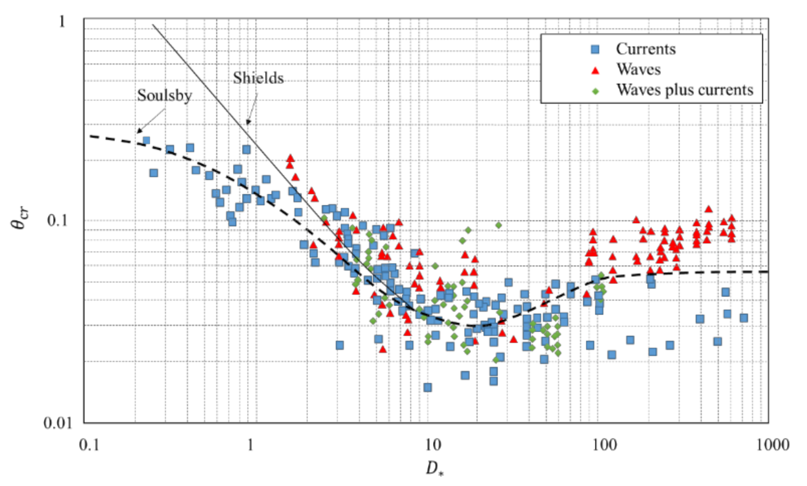
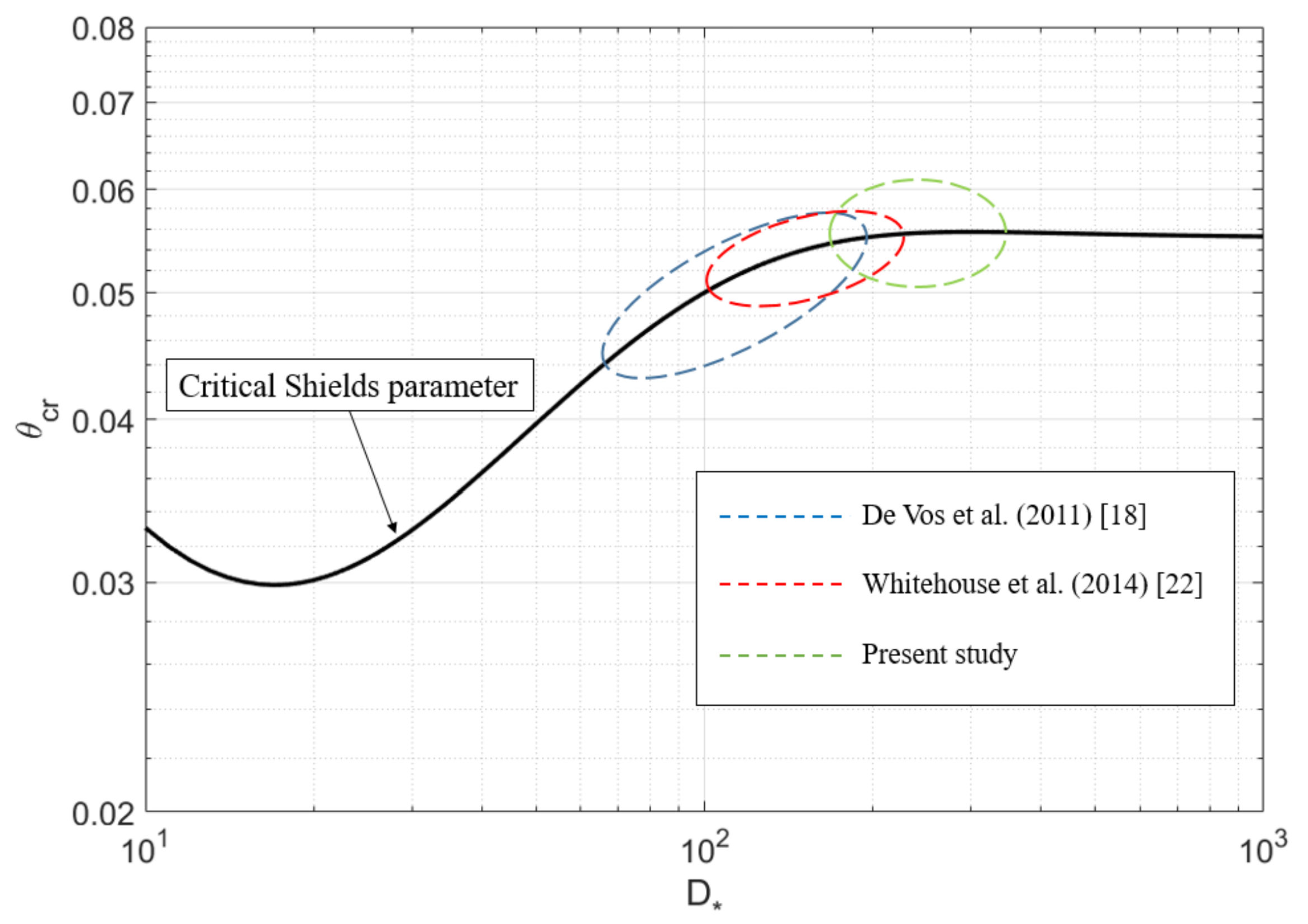
To comply with a consistency of using the Soulsby’s curve for the threshold of the motion (Figure 1), the bed shear stress is also analyzed via Equation (16),

$$f_w=1.39{\left(\frac{A}{z_0}\right)}^{-0.52},$$

(16)

where $A$ is the amplitude of the wave orbital motion at the bed. For regular waves, $A=H/2sinh\left(kd\right)$, $k$ is the wave number. For irregular waves, $A=U_{m}T/2\pi$ and $U_m=\sqrt{2}{U}_{rms}$ [38].

Regarding the bed shear stress for a combined waves and currents conditions, [44] proposes a simple and explicit formula by using a direct fit of laboratory and field measurements in order to compute the maximum shear stress ${\tau }_{max}$, which is known as the DATA2 method, as shown in Equations (17) and (18).

$${\tau }_m={\tau }_c\left[1+1.2{\left(\frac{{\tau }_w}{{\tau }_w+{\tau }_c}\right)}^{3.2}\right],$$

(17)

$${\tau }_{max}={\left({\left({\tau }_m+{\tau }_w\left|cos \varphi \right|\right)}^2+{\left({\tau }_w\left|sin \varphi \right|\right)}^2\right)}^{0.5},$$

(18)

The corresponding shear velocities are then defined with Equations (19)–(21).

$$u_{*c}=\sqrt{\frac{{\tau }_c}{\rho }},$$

(19)

$$u_{*w}=\sqrt{\frac{{\tau }_w}{\rho }},$$

(20)

$$u_{*max}=\sqrt{\frac{{\tau }_{max}}{\rho }},$$

(21)

The result of the bed shear stress analysis is shown in

Table 3. Bed shear stress analysis results.

Test ID	Bed Friction Coefficient Due to Current	Bed Shear Stress, Current	Bed Friction Coefficient Due to Waves [43]	Bed Friction Coefficient Due to Waves [38]	Bed Shear Stress, Waves [43]	Bed Shear Stress, Waves [38]	Max. Bed Shear Stress	Shear Velocity Current	Shear Velocity Waves	Max. Shear Velocity
	${\mathit{f}}_{\mathit{c}}$	${\mathit{\tau }}_{\mathit{c}}$	${\mathit{f}}_{\mathit{w}}$	${\mathit{f}}_{\mathit{w}}$	${\mathit{\tau }}_{\mathit{w}}$	${\mathit{\tau }}_{\mathit{w}}$	${\mathit{\tau }}_{\mathit{m}\mathit{a}\mathit{x}}$	${\mathit{u}}_{*\mathit{c}}$	${\mathit{u}}_{*\mathit{w}}$	${\mathit{u}}_{*\mathit{m}\mathit{a}\mathit{x}}$
	Equation (14)	Equation (10)	Equation (15)	Equation (16)	Equation (11)		Equation (18)	Equation (19)	Equation (20)	Equation (21)
	(-)	(N/m2)	(-)	(-)	(N/m2)	(N/m2)	(N/m2)	(m/s)	(m/s)	(m/s)
Test 03A	8.74 × 10−3	0.273	1.07 × 10−1	1.16 × 10−1	3.700	4.029	4.314	0.017	0.063	0.066
Test 03B	8.74 × 10−3	0.273	8.94 × 10−2	1.04 × 10−1	4.822	5.582	5.862	0.017	0.075	0.077
Test 03C	8.74 × 10−3	0.273	9.15 × 10−2	1.05 × 10−1	4.659	5.350	5.630	0.017	0.073	0.075
Test 03D	8.74 × 10−3	0.273	9.86 × 10−2	1.10 × 10−1	5.918	6.619	6.897	0.017	0.081	0.083
Test 03E	8.74 × 10−3	0.273	8.63 × 10−2	1.01 × 10−1	7.185	8.422	8.698	0.017	0.092	0.093
Test 05A	6.74 × 10−3	0.259	8.24 × 10−2	9.82 × 10−2	1.619	1.929	2.236	0.016	0.044	0.047
Test 05B	6.74 × 10−3	0.259	7.49 × 10−2	9.23 × 10−2	1.850	2.279	2.573	0.016	0.048	0.051
Test 05C	6.74 × 10−3	0.259	6.33 × 10−2	8.27 × 10−2	2.367	3.091	3.370	0.016	0.056	0.058
Test 05D	6.74 × 10−3	0.259	5.72 × 10−2	7.74 × 10−2	2.757	3.732	4.005	0.016	0.061	0.063
Test 05E	6.74 × 10−3	0.259	5.31 × 10−2	7.38 × 10−2	3.072	4.267	4.537	0.016	0.065	0.067
Test 05F	6.74 × 10−3	0.259	6.99 × 10−2	8.82 × 10−2	2.788	3.518	3.792	0.016	0.059	0.062
Test 05G	6.74 × 10−3	0.259	6.47 × 10−2	8.39 × 10−2	3.220	4.174	4.444	0.016	0.065	0.067
Test 07A	7.20 × 10−3	0.201	5.89 × 10−2	7.89 × 10−2	2.622	3.514	3.727	0.014	0.059	0.061
Test 07C	7.20 × 10−3	0.201	6.62 × 10−2	8.51 × 10−2	3.123	4.017	4.228	0.014	0.063	0.065
Test 07D	7.20 × 10−3	0.201	6.02 × 10−2	8.00 × 10−2	3.590	4.773	4.980	0.014	0.069	0.071
Test 09A	7.87 × 10−3	0.225	7.25 × 10−2	9.03 × 10−2	2.750	3.426	3.665	0.015	0.059	0.061
Test 09B	7.87 × 10−3	0.225	8.75 × 10−2	1.02 × 10−1	2.941	3.430	3.669	0.015	0.059	0.061
Test 09C	7.87 × 10−3	0.225	7.62 × 10−2	9.33 × 10−2	3.580	4.384	4.617	0.015	0.066	0.068
Test 11A	7.87 × 10−3	0.620	6.15 × 10−2	8.12 × 10−2	6.959	9.181	9.805	0.025	0.096	0.099
Test 11B	7.87 × 10−3	0.620	8.00 × 10−2	9.63 × 10−2	4.752	5.719	6.350	0.025	0.076	0.080
Test 11C	7.87 × 10−3	0.620	7.20 × 10−2	8.99 × 10−2	5.564	6.948	7.575	0.025	0.083	0.087
Test 11D	7.87 × 10−3	0.620	5.88 × 10−2	7.88 × 10−2	7.546	10.117	10.741	0.025	0.101	0.104
Test 11E	7.87 × 10−3	0.620	9.70 × 10−2	1.09 × 10−1	5.357	6.028	6.658	0.025	0.078	0.082
Test 11F	7.87 × 10−3	0.620	8.82 × 10−2	1.03 × 10−1	6.139	7.142	7.769	0.025	0.085	0.088
Test 11G	7.87 × 10−3	0.620	8.28 × 10−2	9.84 × 10−2	6.828	8.121	8.747	0.025	0.090	0.094
Test 11H	7.87 × 10−3	0.620	7.49 × 10−2	9.23 × 10−2	7.803	9.609	10.234	0.025	0.098	0.101
Test02B	8.74 × 10−3	0.621	2.20 × 10−1	1.86 × 10−1	1.740	1.469	2.194	0.025	0.038	0.047
Test04B	8.74 × 10−3	1.084	1.70 × 10−1	1.57 × 10−1	2.601	2.407	3.548	0.033	0.049	0.060
Test06B	6.74 × 10−3	0.454	1.34 × 10−1	1.35 × 10−1	1.279	1.286	1.859	0.021	0.036	0.043
Test08B	7.20 × 10−3	0.886	1.21 × 10−1	1.26 × 10−1	1.217	1.267	2.268	0.030	0.036	0.048
Test10B	7.87 × 10−3	0.428	1.49 × 10−1	1.44 × 10−1	1.412	1.366	1.902	0.021	0.037	0.044
Test12B	7.87 × 10−3	1.023	1.28 × 10−1	1.31 × 10−1	3.400	3.470	4.528	0.032	0.059	0.067
Test13B	8.34 × 10−3	1.354	1.87 × 10−1	1.67 × 10−1	3.103	2.776	4.178	0.037	0.053	0.065

. It can be seen that the bed shear stress due to waves gives the main contribution to the maximum bed shear stress in the regular wave cases. For the irregular wave cases, the bed shear stress due to the steady flow also plays an important role.

4.2. Static Stability Analysis

During the experiments, the threshold of motion is detected by visual observation via the underwater camera. This visual observation method has been used in both [18,25], where the reliability is discussed in detail by the latter reference. However, for the visual assessment of the present experiments, the visibility is affected by the sand suspension, therefore only very clear rock movement is observed.

The static stability analysis approach is thoroughly explained in [18] while the regression formula for a pile model of $D_P$ = 0.1 m is given in Equation (7). For the tests using a $D_P=0.3$ m model, the predicted critical bed shear stress ${\tau }_{cr,pred}$ can be calculated via Equation (22). Further, for tests using a $D_P$ = 0.6 m model, ${\tau }_{cr,pred}$ is calculated by Equation (23).

$${\tau }_{cr,pred}=4.997+3.569{\tau }_c+0.765{\tau }_w,$$

(22)

$${\tau }_{cr,pred}=9.954+3.569{\tau }_c+0.765{\tau }_w$$

(23)

The regression in [18] applied the critical bed shear stress using a stone size of $D_{67.5}$ and a critical Shields parameter of ${\theta }_{cr}$ = 0.035, which leads ${\tau }_{cr,2}$ as expressed in Equation (24).

$${\tau }_{cr,2}=0.035\rho g\left(s-1\right)D_{67.5}$$

(24)

A comparison between Equations (24) and (3) is introduced by [45]. The experimental results and predicted shear stresses are presented in

Table 4. Static stability analysis results.

Test ID	Predicted Critical Shear Stress	Critical Bed Shear Stress [37]	Critical Bed Shear Stress [18]	Critical Shields Parameter [37]	Maximum Shields Parameter [44]	Stab Parameter	Dimension-Less Diameter	Clear Rock Motion Noticed?
	${\mathit{\tau }}_{\mathit{c}\mathit{r},\mathit{p}\mathit{r}\mathit{e}\mathit{d}}$	${\mathit{\tau }}_{\mathit{c}\mathit{r}}$	${\mathit{\tau }}_{\mathit{c}\mathit{r},2}$	${\mathit{\theta }}_{\mathit{c}\mathit{r}}$	${\mathit{\theta }}_{\mathit{m}\mathit{a}\mathit{x}}$	Stab	${\mathit{D}}_{*}$	$\mathbf{Yes}/\mathbf{No}$
	Equation (22)–(23)	Equation (3)	Equation (24)	Equation (2)	Equation (6)	Equation (5)	-	-
	(N/m2)	(N/m2)	(N/ m2)	(-)	(-)	(-)	(-)	(-)
Test 03A	8.803	11.268	8.943	0.056	0.021	0.383	290	No
Test 03B	9.661	11.268	8.943	0.056	0.029	0.520	290	No
Test 03C	9.536	11.268	8.943	0.056	0.028	0.500	290	No
Test 03D	10.499	11.268	8.943	0.056	0.034	0.612	290	No
Test 03E	11.469	11.268	8.943	0.056	0.043	0.772	290	No
Test 05A	7.159	5.921	4.829	0.054	0.020	0.378	157	No
Test 05B	7.336	5.921	4.829	0.054	0.024	0.435	157	No
Test 05C	7.731	5.921	4.829	0.054	0.031	0.569	157	No
Test 05D	8.030	5.921	4.829	0.054	0.037	0.676	157	Yes
Test 05E	8.271	5.921	4.829	0.054	0.042	0.766	157	Yes
Test 05F	8.053	5.921	4.829	0.054	0.035	0.640	157	No
Test 05G	8.383	5.921	4.829	0.054	0.041	0.751	157	Yes
Test 07A	7.719	5.921	4.829	0.054	0.034	0.630	157	No
Test 07C	8.102	5.921	4.829	0.054	0.039	0.714	157	No
Test 07D	8.459	5.921	4.829	0.054	0.046	0.841	157	Yes
Test 09A	7.903	5.921	4.829	0.054	0.034	0.619	157	No
Test 09B	8.049	5.921	4.829	0.054	0.034	0.620	157	Yes
Test 09C	8.538	5.921	4.829	0.054	0.042	0.780	157	Yes
Test 11A	17.490	12.170	9.659	0.056	0.045	0.806	313	No
Test 11B	15.802	12.170	9.659	0.056	0.029	0.522	313	No
Test 11C	16.423	12.170	9.659	0.056	0.035	0.622	313	No
Test 11D	17.939	12.170	9.659	0.056	0.049	0.883	313	Yes
Test 11E	16.264	12.170	9.659	0.056	0.030	0.547	313	No
Test 11F	16.863	12.170	9.659	0.056	0.036	0.638	313	No
Test 11G	17.390	12.170	9.659	0.056	0.040	0.719	313	No
Test 11H	18.136	12.170	9.659	0.056	0.047	0.841	313	Yes

.

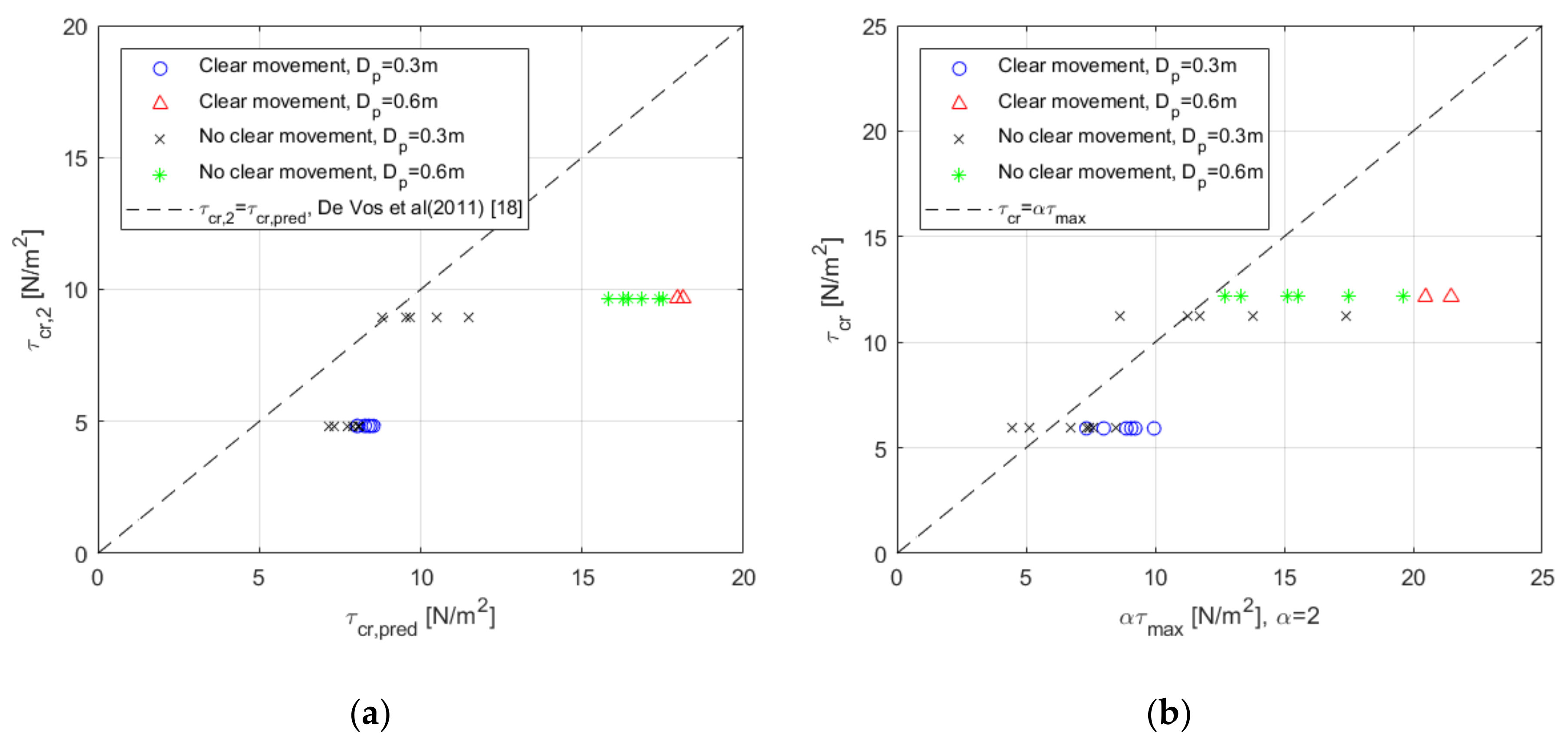
Figure 7a shows the difference between the critical bed shear stress and the predicted bed shear stress using the method of De Vos et al. (2011) [18] (Equations (22)–(24)). From the perspective of onset of motion, Figure 7a shows that the predicted critical bed shear stress for the small scale model introduced in [18] results in a conservative approach. For the cases with $D_P$ = 0.3 m and $D_{50}$ = 6.75 mm, the clear stone movement happens when ${\tau }_{cr,pred}\approx 1.66{\tau }_{cr,2}$. For the cases with $D_P$ = 0.6 m and $D_{50}$ = 13.5 mm, the clear stone movement happens when ${\tau }_{cr,pred}\approx 1.77{\tau }_{cr,2}$. It can be seen that the predicted critical bed shear stress will lead to a conservative value for the large scale ratio. Figure 7b shows the relationship between the local bed shear stress around the pile and the critical bed shear stress via the models of reference [37]. The local bed shear stress is calculated by Equation (3) and determined by assuming a uniform amplification factor $\alpha$ = 2. It is seen that using $\alpha$ = 2 results in a more scattered distribution of the local bed shear stress and a conservative estimation of the threshold of motion.

It should be noted that during the present large-scale tests, a live-bed situation was measured and the sediment suspension made the recorded image blurry after 2–3 waves, which clearly affects the recording quality and the possibility to see initiation of motion. Meanwhile, due to the great distance between the pile and the underwater camera, the motions of very small stones are not able to be captured. It is therefore possible that stone entrainment occurred before it was visually acknowledged, and it is not possible to develop a new formula based on these data. However, it can be noted that the predicted critical shear stress by [18] tends to be on the safe side.

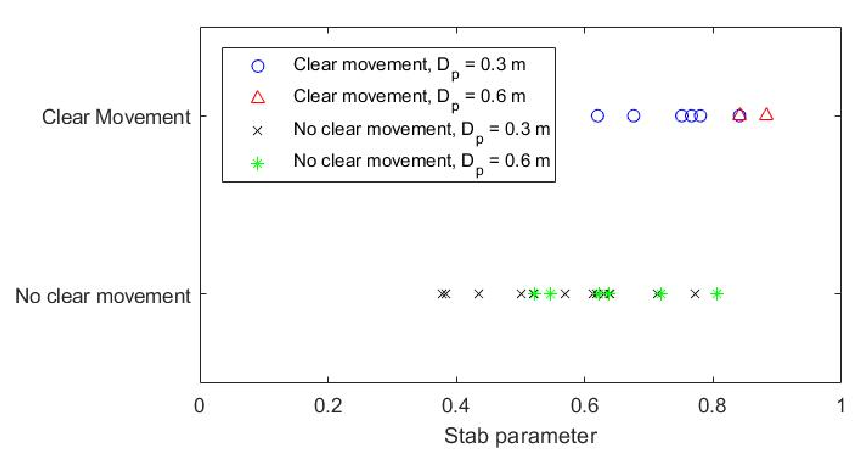
Figure 8 shows the relationship between the Stab parameter (Opti-Pile) and the observed onset of motion based on the camera results. Most of the calculated Stab parameters are in the range of 0.4–0.8. These values, according to reference [17], have exceeded the criteria of a static design, which should trigger the incipient of motion. However, the experimental results show that this judgement could also be conservative and safe, and no clear relationship between the Stab parameter and the threshold of motion was identified for this dataset. Stab parameters of 0.6–0.8 may give a result of either observed stone motion or no motion.

The deviations between the present results of the large scale tests and the existing static design method can be attributed to several reasons. Firstly, the Soulsby’s curve (Figure 1) has a wide dispersion for waves combined with current conditions in the range of $D_{*}$ > 100. This makes it difficult to obtain an accurate analysis for the static analysis. Secondly, scale effects exist as the viscous forces cannot be scaled correctly, and the local amplification factor might be smaller as the model scale increases. Scale effects can also be seen from the Soulsby’s curve. As can be seen in Figure 9, the $D_{*}$ range for various experiments has been plotted. The critical bed shear stress for the present large scale tests are clearly larger than in the previous studies using small scale models, such as [18,22], which means the small scale experiments are more conservative with regard to the incipient of stone motion.

4.3. Dynamic Stability Analysis

Beside the study of the onset of motion, the dynamic stability of the scour protection layer was investigated. A dynamically stable scour protection will result in a much smaller stone size of the protection layer and significantly reduce the cost of the installation, depending on the volume of rock material for a proper thickness of the armor layer.

The large scale tests hereby have cover a wide range of environmental conditions, including different water depths, pile diameters and stone sizes. In order to have a clear insight, dimensionless expressions are necessary to depict the relationship among the combined conditions. The key dimensionless parameters in this situation include the Reynolds numbers for the pile (Equation (25)) and the stones (Equation (26)), the Froude number for the stones (Equation (27)), the Keulegen–Carpenter number (Equation (28)), the ratio between wave and current velocities (Equation (29)), the ratio between water depth and pile diameter ($d/D_P$) and the ratio between stone size and pile diameter ($D_{50}/D_P$).

$$R{e}_{Dp}=\frac{\left(U_m+\left|U_c\right|\right)D_P}{\upsilon }$$

(25)

$$R{e}_{D_{n50}}=\frac{u_{*max}{D}_{n50}}{\upsilon }$$

(26)

$$F{r}_{Dn50}=\frac{\left|U_c\right|}{\sqrt{g{D}_{n50}}}$$

(27)

$$KC=\frac{U_m{T}_P}{D_P}$$

(28)

$$U_{cw}=\frac{\left|U_c\right|}{\left|U_c\right|+U_m}$$

(29)

An overview of the values of these dimensionless parameters for the irregular wave tests are listed in

Table 5. Dimensionless parameters for irregular wave tests.

Test ID	Re Number, Using Pile Diameter	Re Number, Using Stone Diameter	Fr Number Using Stone Diameter	KC Number	Ratio of Velocities	Water Depth to Pile Diameter Ratio	Stone Size to Pile Diameter Ratio	Stab Para-Meter	Predicted S3D Value	Measured S3D Value
	$\mathit{R}{\mathit{e}}_{\mathit{D}\mathit{p}}$	$\mathit{R}{\mathit{e}}_{\mathit{D}\mathit{n}50}$	$\mathit{F}{\mathit{r}}_{\mathit{D}\mathit{n}50}$	$\mathbf{KC}$	${\mathit{U}}_{\mathit{c}\mathit{w}}$	$\mathit{d}/{\mathit{D}}_{\mathit{P}}$	${\mathit{D}}_{\mathit{n}50}/{\mathit{D}}_{\mathit{P}}$	Stab	${\mathit{S}}_{3\mathit{D},\mathit{p}\mathit{r}\mathit{e}\mathit{d}}$	${\mathit{S}}_{3\mathit{D}}$
	Equation (25)	Equation (26)	Equation (27)	Equation (28)	Equation (29)	-	-	Equation (5)	Equation (9)	Equation (8)
Test 02B	1.51 × 105	494	1.175	1.043	0.750	4.0	0.035	0.195	0.75	0.46
Test 04B	2.02 × 105	626	1.552	1.448	0.740	4.0	0.035	0.315	3.09	0.68
Test 06B	1.52 × 105	244	1.556	1.051	0.726	5.0	0.019	0.314	4.28	0.83
Test 08B	1.91 × 105	270	2.103	1.191	0.778	4.0	0.019	0.383	11.52	2.47
Test 10B	1.40 × 105	249	1.399	0.917	0.706	3.0	0.019	0.321	2.38	0.82
Test 12B	4.44 × 105	760	1.529	1.109	0.689	3.0	0.019	0.372	4.22	2.35
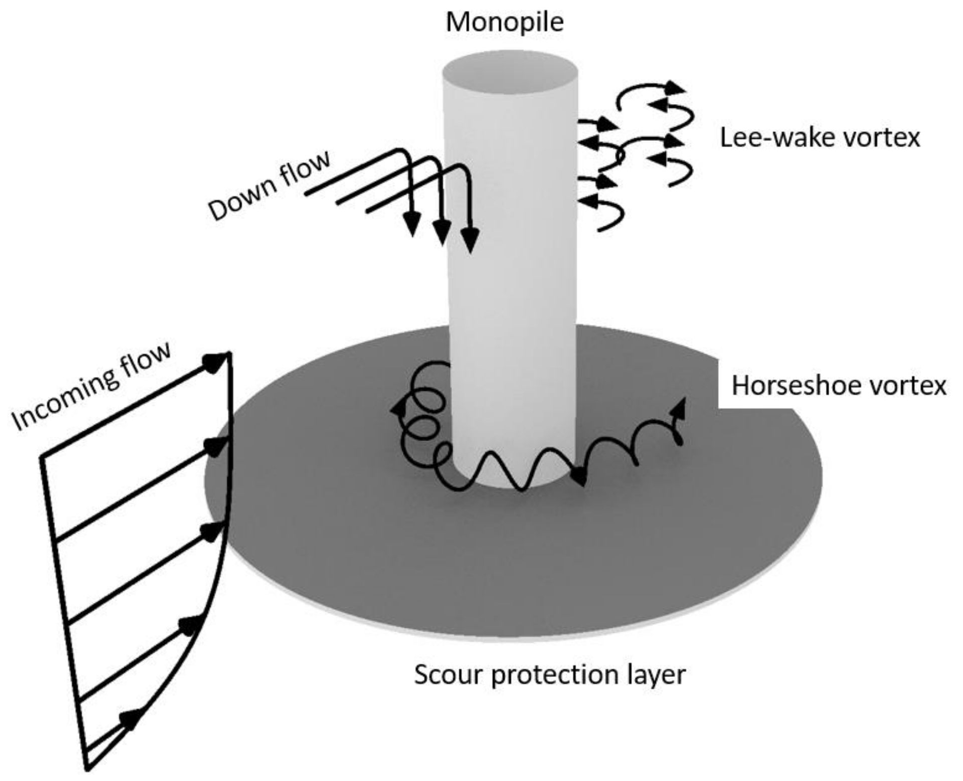
Test 13B	4.51 × 105	737	1.709	0.693	0.758	2.5	0.019	0.343	3.71	1.08

. The dimensionless parameters can indicate the flow properties in the experiments which can determine the formation of flow separation, lee-wake vortexes and horseshoe vortexes. As seen from Table 5, the Reynolds numbers of the pile, $R{e}_{Dp}$, are in the magnitude of O(10⁵), indicating the flow around the pile has a fully turbulent wake [46]. The KC number reflects the effects of the oscillatory flows. In the present experiment, the range of KC number is 0.693 < KC < 1.448, which means the oscillatory flow due to the waves will not lead to severe vortex shedding nor to the development of a horseshoe vortex, but might only introduce a pair of vortices at the wake side of the wave-induced flow, according to [9,46]. The ratio between current and waves, $U_{cw}$, reflects the velocity components of the flow and the wave or current dominated regime, where $U_{cw}$ = 1 gives a current only condition and $U_{cw}$ = 0 is a wave only condition. For all cases shown in Table 5, $U_{cw}$ > 0.689. This means the flow is dominated by the steady current.

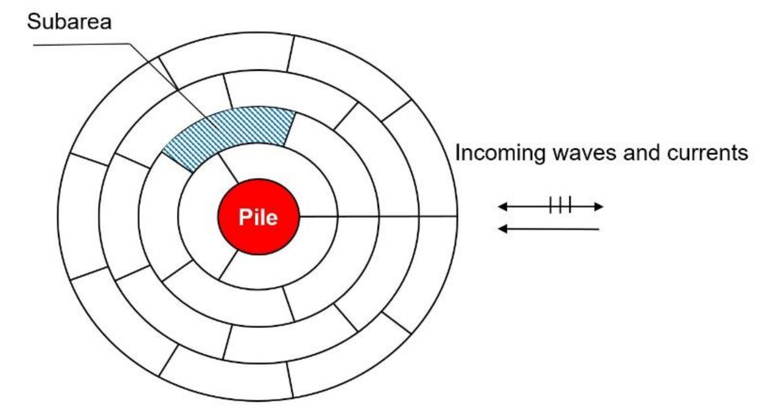
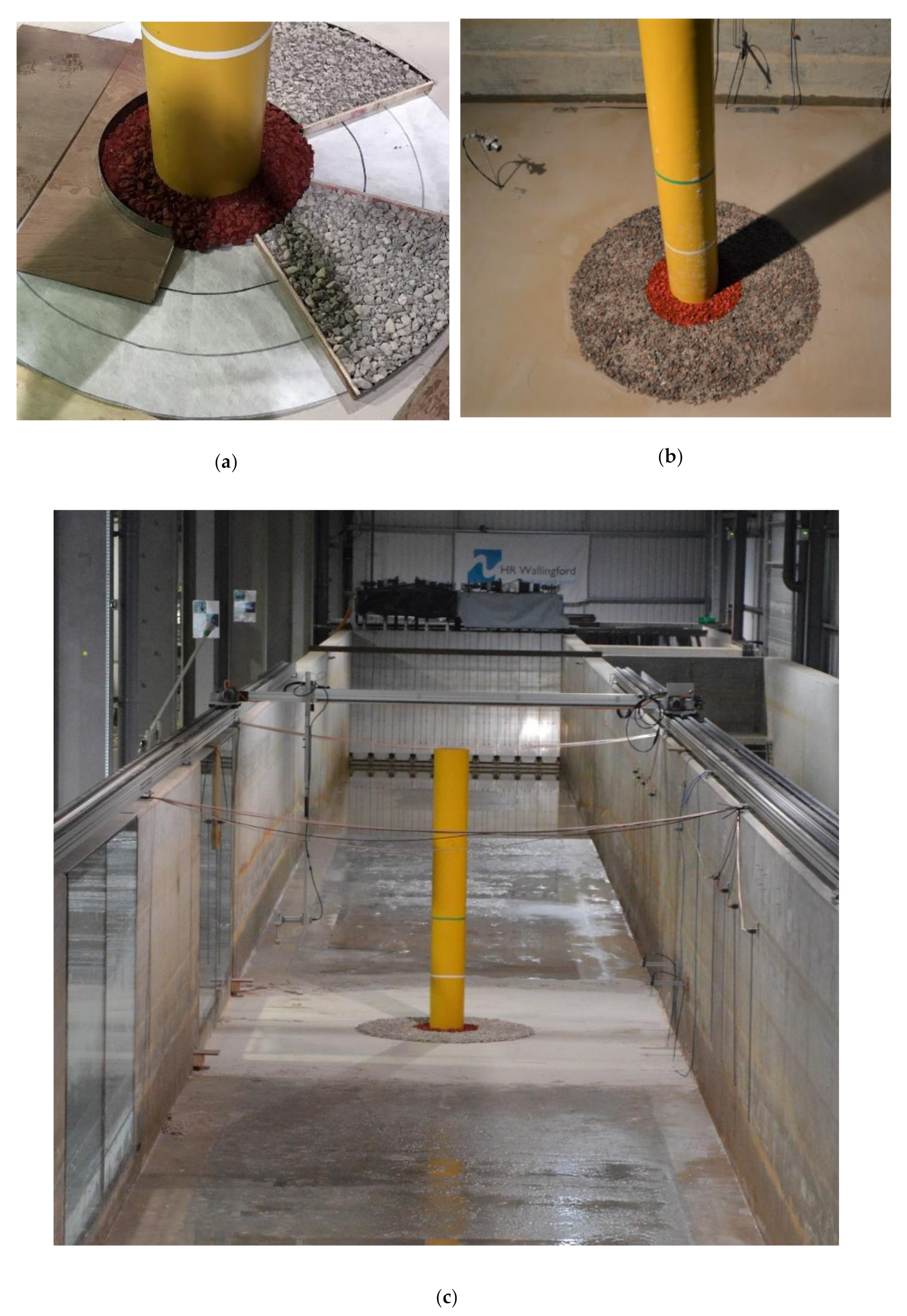
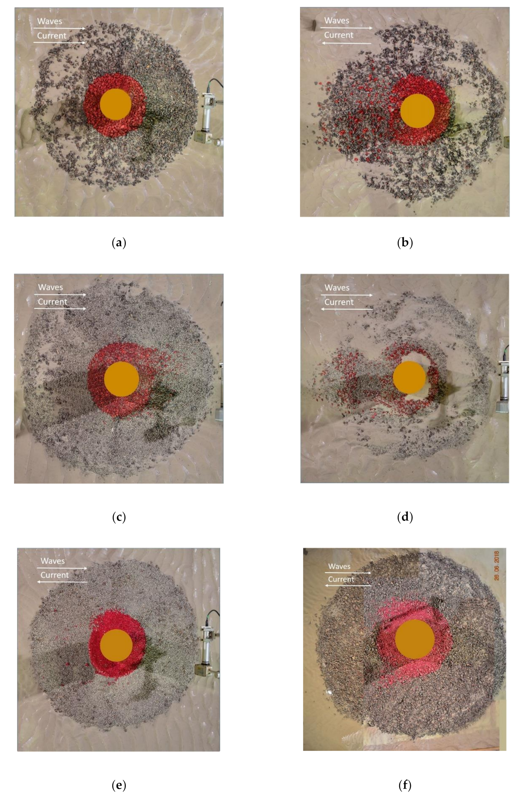
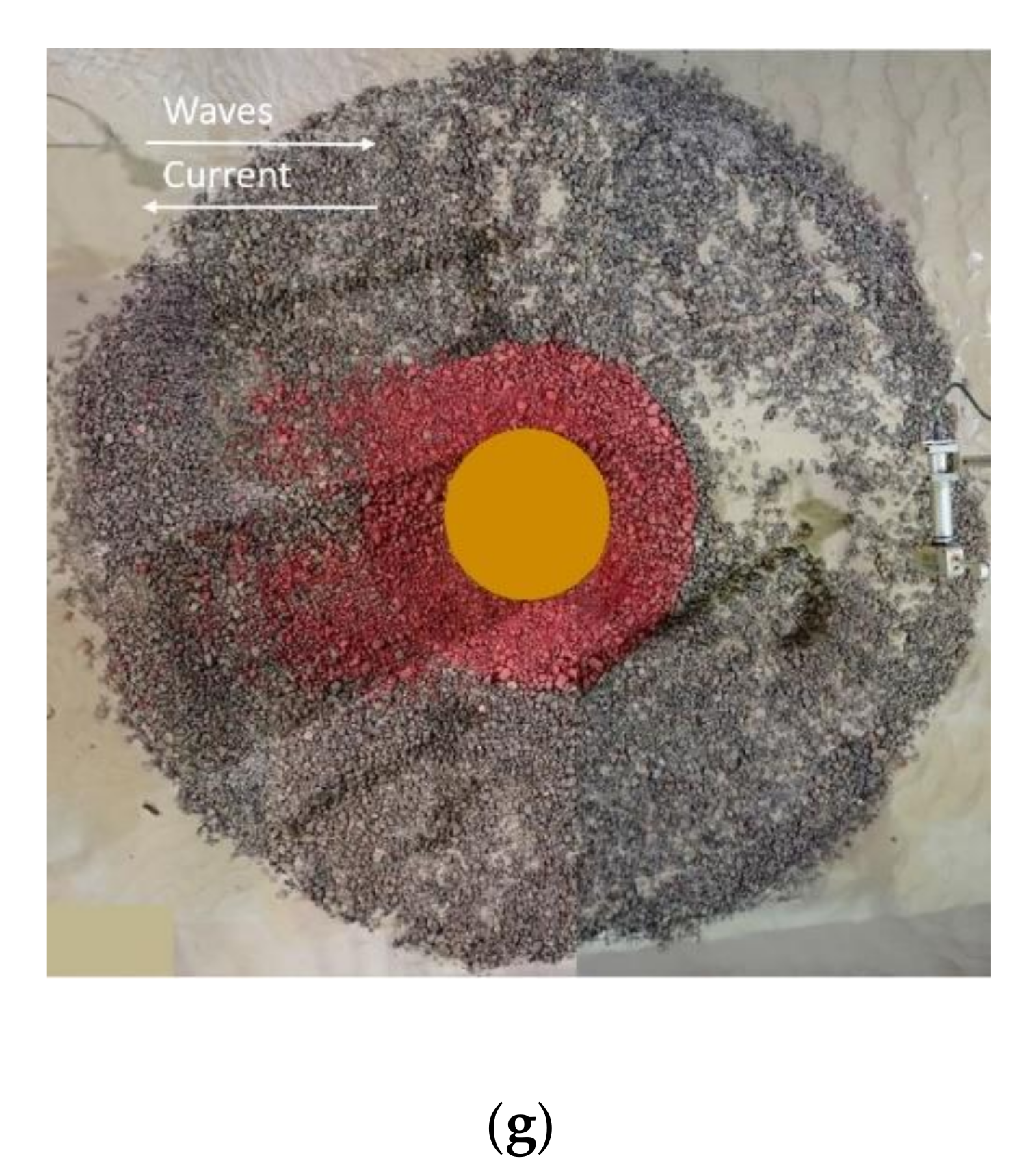
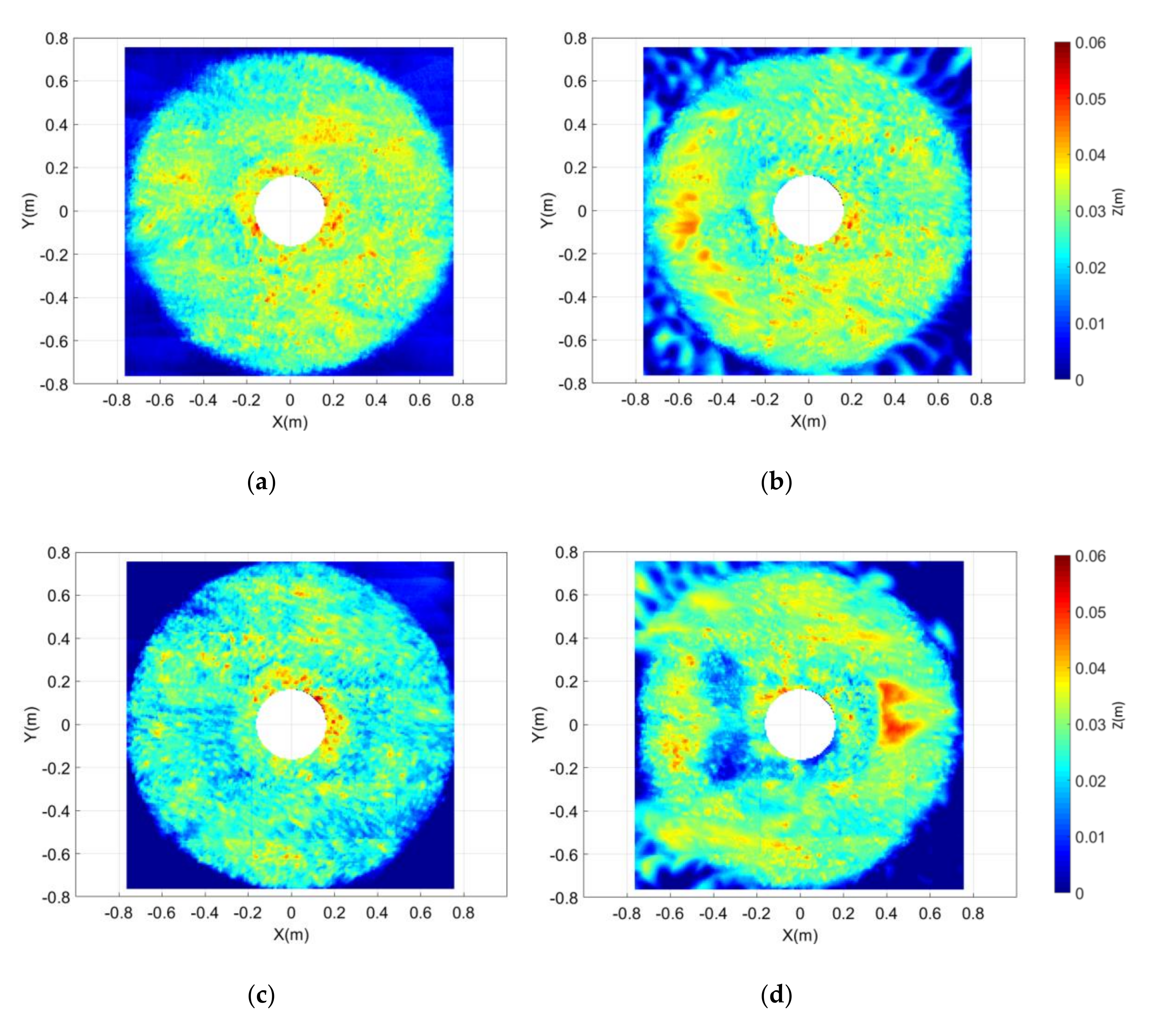
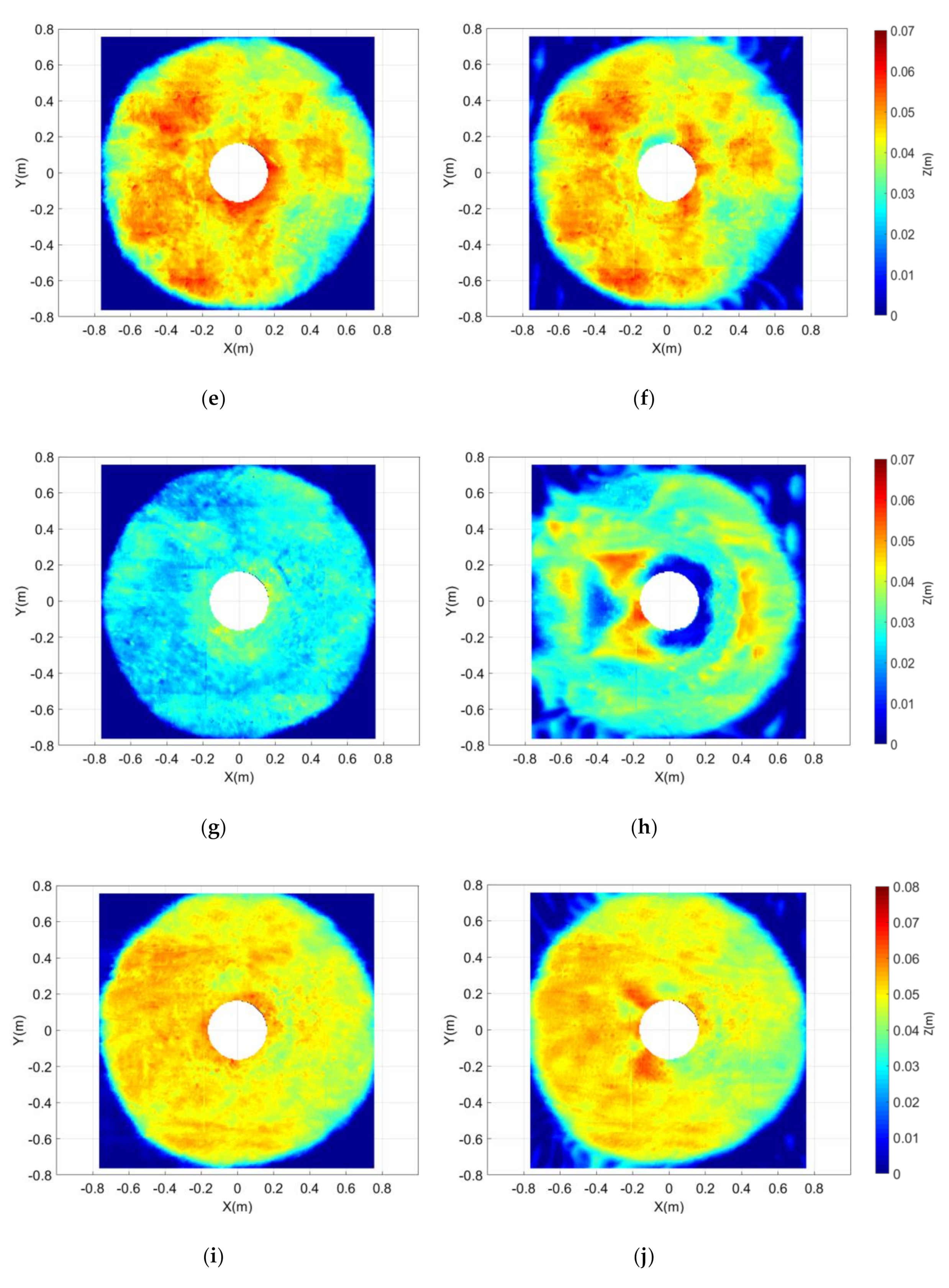
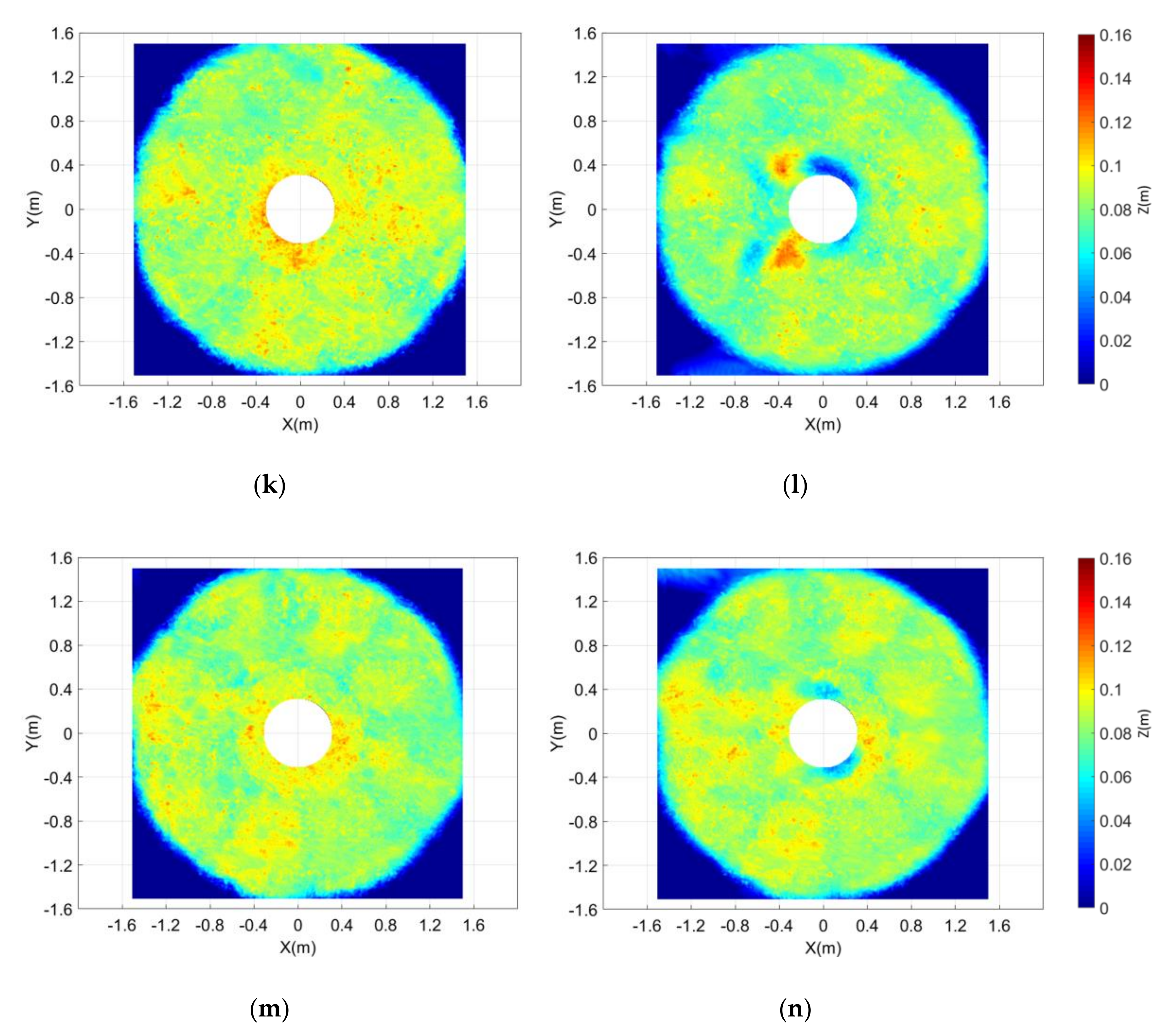
The damage patterns after 3000 waves from the overhead cameras and the corresponding scanned bed surface elevations are displayed in Figure 10 and Figure 11. The red colored stones in the inner ring can clearly show how they are transported by the flow around the pile due to the waves and the current. In most of the cases, significant horseshoe vortices and lee-wake vortices due to the current can be noticed as the inner ring stones are moved by the hydrodynamic loads and form a wake shape in the downstream of the pile. The removal of the inner ring stones leads to an erosion pattern nearby the pile at a ±45° position towards the incoming current, for example, in Test 04B, 08B, 12B, and 13B. The observed phenomena are in accordance with [47], where the maximum amplification factor also occurs at ±45° position towards to the incoming flow. For Test 08B, the protection fails as many inner ring rocks are removed and the geotextile is exposed. For Test 02B, the removal of inner ring rocks is not obvious as the hydrodynamic load is relatively week.

The Stab parameter (Equation (5)) and the measured and predicted $S_{3D}$ (Equations (8) and (9)) values are also given in Table 5. For the present cases, the Stab parameter is always less than 0.4. The protection layer is assumed to be statically stable [17]. However, it can be seen that most of the presented results are clearly not statically stable but dynamically stable. This shows the design limitation of using the predicted Stab parameter as an underestimation of the damage level.

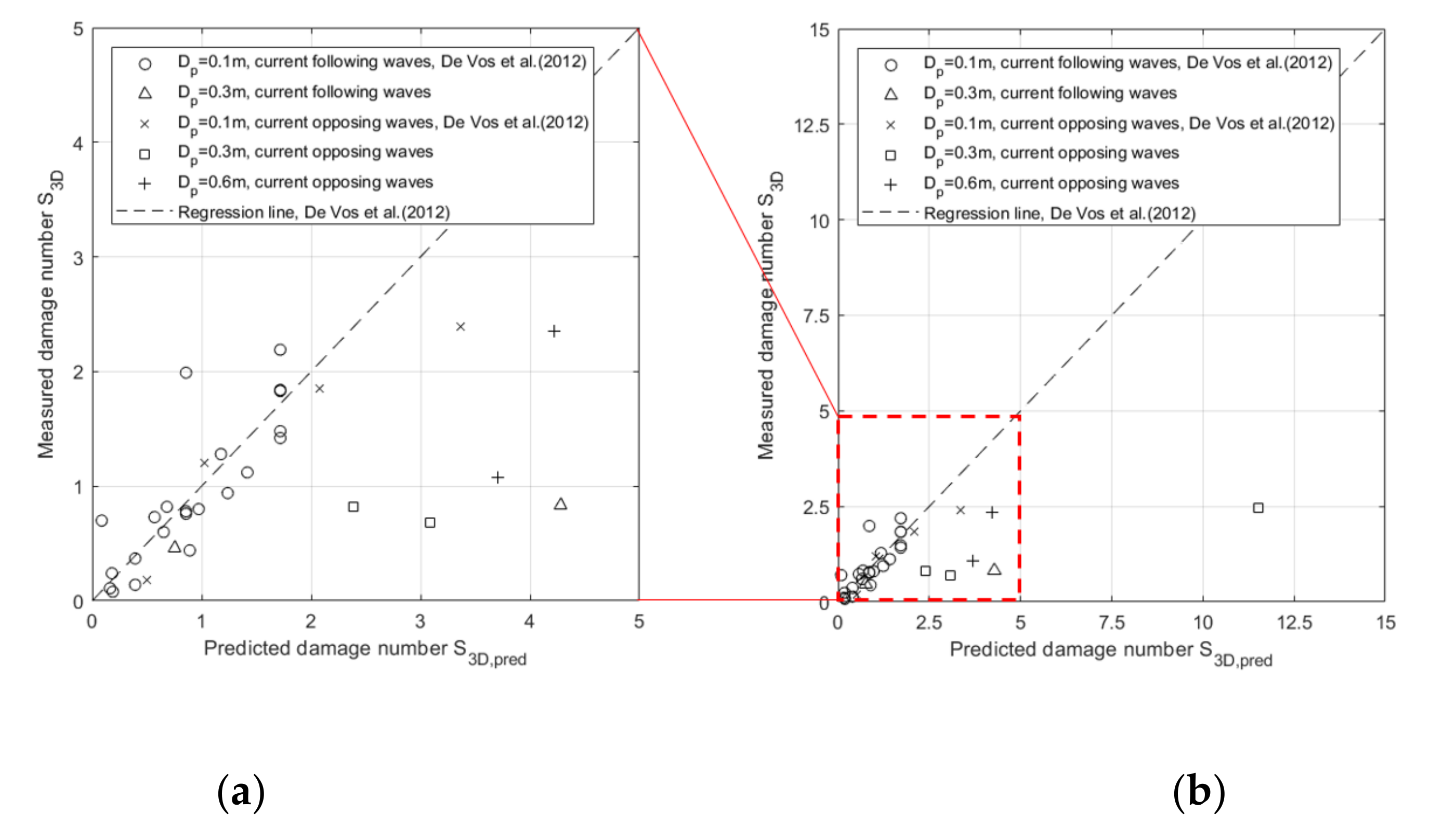
A comparison is made between predicted and measured $S_{3D}$ values after 3000 waves as shown in Figure 12. It can be noted that the predicted damage numbers are almost larger than the measured damage numbers, regardless of whether waves are following or opposing current. It is defined by De Vos et al. (2012) [19] that failure occurs when the estimated damage number is larger than 1. However, despite Test 08B, no clear failure is seen in Test 02B, 04B, 06B, 10B, 12B, and 13B, despite the predicted damage numbers $S_{3D,pred}$ being larger than 2. For Test 08B, the damage pattern shows a clear horseshoe vortex induced by the current, causing a large exposure area of the geotextile. The high damage number is mainly due to the high current condition, the small stone material, and a lower protection layer thickness.

The results show that Equation (9) will give a conservative prediction of the dynamic stability of the scour protection layer. Several reasons may lead to the deviations between the predicted values and the measured values. One key reason might be that the large scale experimental conditions are out of range for the input parameters in the regression formula (Equation (9)), especially the stone size ($D_{50})$ and the ratio between velocities ($U_{cw}$).

Table 6. The median armor material sizes $D_{50}$ used in different scale tests

Test Series	$$\mathbf{Pile} \mathbf{Diameter} {\mathit{D}}_{\mathit{P}}$$	$$\mathbf{Model} {\mathit{D}}_{50}$$	$$\mathbf{Prototype} {\mathit{D}}_{50}$$	$${\mathit{U}}_{\mathit{c}\mathit{w}}$$
	(m)	(mm)	(mm)	(-)
De Vos et al. (2012) [19]	0.1	4.2–8.6	208–430	0.26–0.70
Test 02B–10B	0.3	6.75–12.5	113–208	0.71–0.78
Test 12B, 13B	0.6	13.5	113	0.69–0.76

shows the difference between the parameters in the present experiments and the experiments of [19]. The applied stone sizes in the present experiments are smaller than in the study of [19] and the experiments presented in this paper focuses on the current dominated flow, $U_{cw}$ > 0.69, which is larger than in most of the test cases in the experiments of [19]. Another reason might be that the layer thicknesses exceeds the ones which were tested in [19]. Other possible reasons can be the scale effects, model effects and experimental uncertainties.

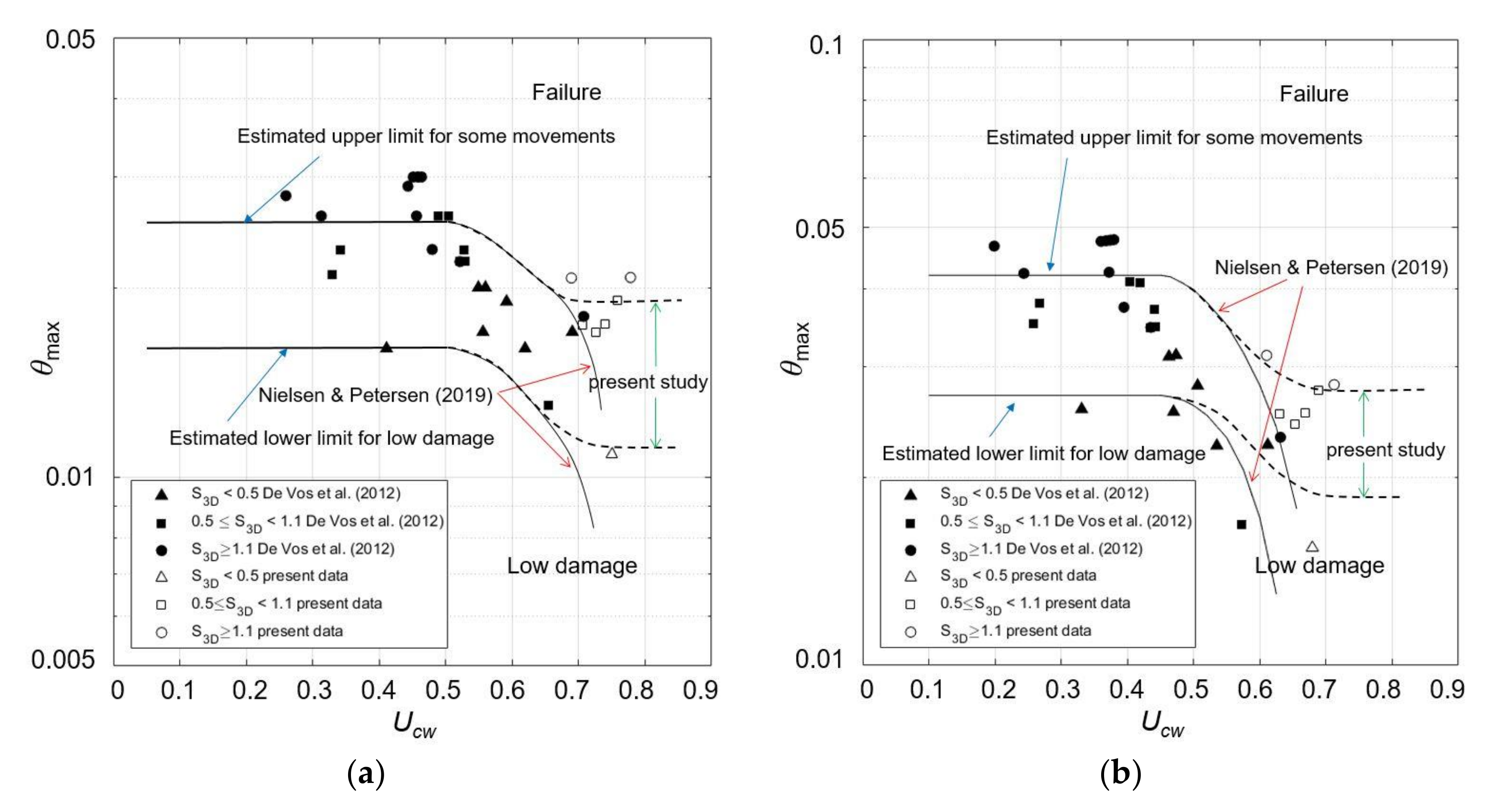
Nielsen and Petersen (2019) [25] proposed a new estimation approach by considering the relationship between the maximum bed shear stress ${\theta }_{max}$, the damage number $S_{3D}$ and the relative velocity $U_{cw}$. The research suggests two estimated limits for low damage and failure, as the solid lines shown in Figure 13. ${\theta }_{max}$ is calculated using $U_m$ in Figure 13a and using $U_s$ (significant value) in Figure 13b. To obtain these values, the small-scale experimental data of De Vos et al. (2012) [19] are analyzed for the estimated limits with $U_{cw}$ < 0.7. As a complement to the dataset, the large scale experimental data with 0.69 < $U_{cw}$ < 0.75 presented in this paper are added to the figure. Although some differences exist when using different wave orbital velocities to calculate ${\theta }_{max}$, the limit lines of ${\theta }_{max}$ for high $U_{cw}$ conditions do not drop dramatically after $U_{cw}$ > 0.5 as given by [25], but stay stable even when $U_{cw}$ > 0.7. This shows that the large scale scour protection can endure a relatively higher bed load than expected. As there is a lack of data regarding how small scale tests behave in very high $U_{cw}$ conditions, it is not easy to draw a fair conclusion regarding the scale effects, and therefore more investigations are expected in a future study to overcome this lack of knowledge.

4.4. Erosion Depth of Scour Protection Layer

The erosion depth is an important parameter to depict the damage of the scour protection. De Schoesitter et al. (2014) [21] discussed that using more layers of smaller size stones will reduce the rate of failure of a scour protection. The failure is defined as the exposure of filter with an area of $4D_{50}{}^2$. This is equivalent to an area of four adjacent stones removed in the bottom of the armor layer. However, this definition is quite sensitive to the randomness of the observation, since the area of exposure is usually rather small compared to the whole area of protection. To the safe side of this definition, it can be understood as the moment when the maximum depth of damage exceeds the thickness of the protection layer. This approach varies from De Vos et al. (2012) [19], as it focuses on erosion depth instead of erosion volume and because the protection layer thickness used in the present large scale test (up to 9$D_{n50}$) is much larger than $3D_{n50}$. Therefore, an investigation of the maximum damage depth of the protection layer can give interesting results.

The principles of the erosion of a scour protection layer under waves and currents is very similar to the scour itself. The discussion of scour depth around a monopile can be found in literature, where the most widely used formula is given in [48] as below (Equations (30)–(32)),

$$\frac{S}{D_P}=\frac{s_c}{D_P}\left\{1-exp\left[-A\left(KC-B\right)\right]\right\},$$

(30)

where $KC\ge 4$ and

$$A=0.03+\frac{3}{4}{U}_{cw}{}^{2.6},$$

(31)

$$B=6exp\left(-4.7U_{cw}\right),$$

(32)

where $S_c$ is the scour depth in steady current alone condition, the mean value for live-bed conditions is $S_c/D_P$ = 1.3 and the standard deviation is 0.7. For low KC numbers, Rudolph and Bos (2006) [49] proposed a modified scour depth prediction equation in the current combined wave conditions, which is fitted using a series of experimental data within the range of 1 < KC < 10, as shown in Equations (33)–(36).

$$\frac{S}{D_P}=1.3\left\{1-exp\left[-A\left(KC-B\right)\right]·{\left(1-U_{cw}\right)}^C\right\},$$

(33)

$$A=0.03+1.5U_{cw}{}^4,$$

(34)

$$B=6exp\left(-5U_{cw}\right),$$

(35)

$$C=0.1,$$

(36)

Qi and Gao (2014) [50] carried out experiments with $0.4<KC<4$ and they found that the dimensionless scour depth is smaller, but still significant when $U_{cw}\ge 0.6$. As the rock material is often quite large when compared to the fine sediments, the undisturbed bed shear stress must be smaller than the critical bed shear stress ($\theta \le {\theta }_{cr}$), which is considered to be a clear water condition. The clear water condition scour depth under steady current was analyzed by Raudkivi and Ettema (1983) [51]. However, for the damage depth of scour protection layer, there remains a scarcity of experimental data under low KC number, wave-plus-current, and clear water conditions.

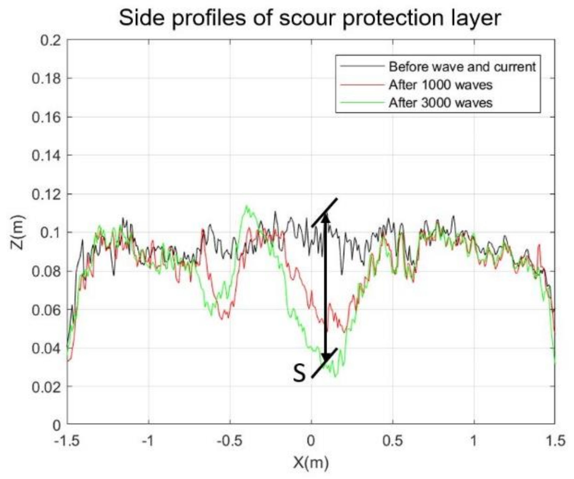
With regards to the maximum damage depth of this scour protection layer, $S$, the definition is similar to that in scour problem. This depth is defined as the maximum eroded height of the scanned profile before and after actions of current and 3000 waves, as shown in Figure 14. In order to ascertain a better insight into the relationship between the maximum damage depth of the scour protection layer around a monopile and the hydrodynamic load due to combined waves and currents conditions, an analysis is carried out based on the large-scale experimental data. The results are shown in

Table 7. Maximum damage depth in present large scale test.

Test ID	Average Armor Layer Thickness	Maximum Damage Depth of Scour Protection	Ratio between Maximum Shear Velocity and Critical Shear Velocity	Dimensionless Damage Depth of Scour Protection	Ratio between Maximum Scour Depth and Average Layer Thickness
	h	$\mathbf{S}$	${\mathit{u}}_{*\mathit{m}\mathit{a}\mathit{x}}/{\mathit{u}}_{\mathit{c}\mathit{r}}$	$\mathit{S}/{\mathit{D}}_{\mathit{P}}$	S/h
	(mm)	(mm)	(-)	(-)	(-)
Test 02B	24.6	24.2	0.441	0.081	0.984
Test 04B	30.0	34.3	0.561	0.114	1.143
Test 06B	49.6	20.8	0.560	0.069	0.419
Test 08b	31.8	37.5	0.619	0.125	1.179
Test 10B	51.4	18.4	0.567	0.061	0.358
Test 12B	92.4	82.9	0.610	0.138	0.897
Test 13B	93.9	76.2	0.586	0.127	0.812

.

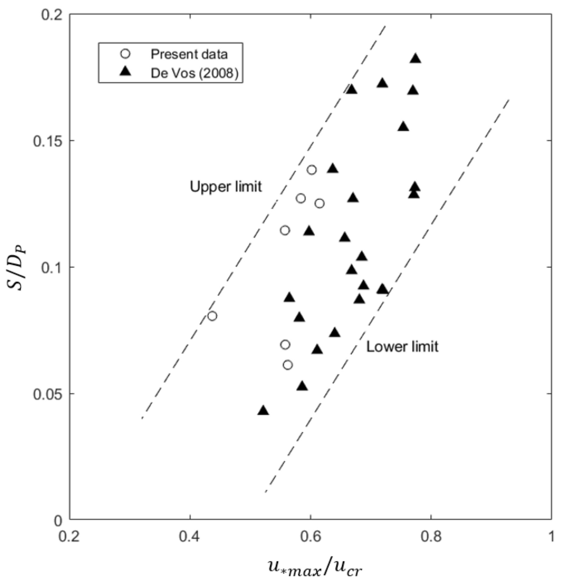
The effect of the ratio between maximum shear velocity and critical shear velocity, $u_{*max}/u_{cr}$ and the Reynolds number of stone size, $R{e}_D$, are plotted in Figure 15 and Figure 16, respectively. As a complement of the data and a comparison between small scale and large scale results, the re-analyzed scanning data from De Vos (2008) [52] is also added to the figures. It is clearly seen that the dimensionless maximum damage depth $S/D_P$ increases as $u_{*max}/u_{cr}$ increases, for both present result and [52]. The maximum depth to pile ratio, $S/D_P$, is mostly bounded between an upper limit and a lower limit with a range of 0.11, approximately. Using Equations (5) and (21), it can be derived that $u_{*max}/u_{cr}=\sqrt{Stab}$. This shows that Stab parameter can reflect the main physics, but is too rough when predicting the damage of the scour protection.

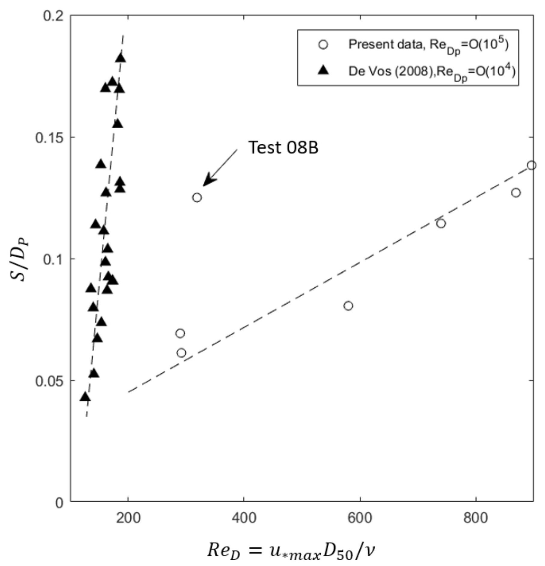
From another perspective, as shown in Figure 16 it is seen that the damage depth increases with the stone Reynolds numbers, $R{e}_D$ ($R{e}_D=1.19{Re}_{Dn50}$, based on the relationship between $D_{n50}$ and $D_{50}$). This is easy to explain as a larger bed shear stress or shear velocity will physically introduce a larger amount of rock material removal. For the present large scale tests, $R{e}_{Dp}~O\left({10}^5\right)$, $S/D_P$ increases slowly as ${Re}_D$ increases, while for the small scale tests, $R{e}_{Dp}~O\left({10}^4\right)$, $S/D_P$ increases sharply as ${Re}_D$ slightly increases. This corresponds to reference [36] which stated that for $R{e}_D$ > 400, the critical bed shear stress is approaching a constant value and is much larger than when $R{e}_D$ < 200. Moreover, this may also be attributed to the horseshoe vortex behaviors in different scales. As in low Re number but turbulent flow condition, the turbulent boundary layer thickness to pile size ($\delta /D_p$) is usually larger, which can cause a larger relative separation distance of the horseshoe vortex [9]. As the flow details are not captured in these experiments, more discussions related to the microscopic interactions between flow and rock material shall be addressed in the future. Nevertheless, the scale effects due to the pile Reynolds number ($R{e}_{Dp}$) are clearly reflected. One exception is Test 08B which shows a significant failure. As listed in Table 5, the stone Froude number for Test 08B is $F{r}_{Dn50}$ = 2.103 and $U_{cw}$ = 0.778. These values are much larger than the values of the other test cases and could be the reason for the large deviation of $S/D_P$ in Figure 16.

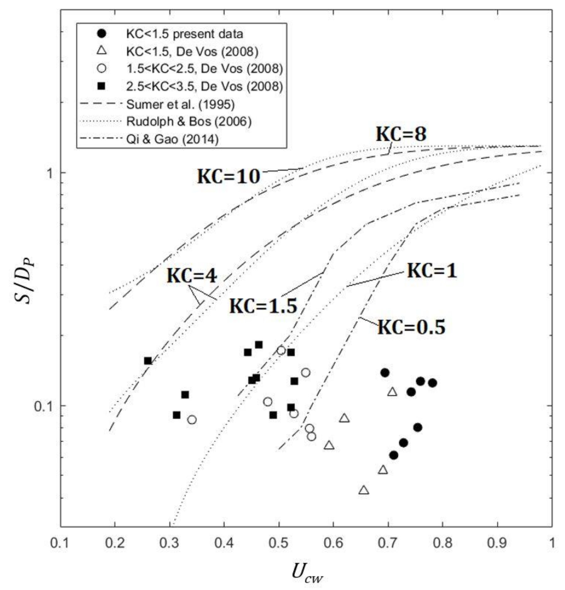
In comparison with the existing models which predict the scour depth in sand under low KC number, the dimensionless damage depth versus $U_{cw}$ is plotted in Figure 17. The regression lines from [48,49,50] are plotted as well for reference. The experimental data from the present large scale tests and De Vos (2008) [52] are categorized by different KC number ranges. All of these data points are within the range of KC < 3.5. It can be seen from the figure that the measured $S/D_P$ are mostly smaller than the predictions. When $U_{cw}$ < 0.4, several data points can be well fitted to the three regression models, but when $U_{cw}$ > 0.4, most of the data points are not able to be fitted ideally, especially for the conditions when KC < 1.5. There are several reasons which could explain the discrepancies between the present experimental data and the existing prediction models. In the first place, the existing formulas are mostly valid for live-bed conditions. It is not clear yet whether the prediction methods are also valid for the scour protection materials in clear water conditions. However, according to the study of [51] on the current-only scour depth in clear water conditions, the scour depth in clear water conditions is less than that in live-bed conditions. This conclusion could be reasonably expanded to the combined waves and current conditions. Secondly, the sediments used in [48,49,50] are fine or coarse sands with small diameters, which results in a different scaling factor for sediment, $N_d=N_l{}^{0.25}$. This is different from the present study where the armor stones are scaled geometrically, $N_d=N_l$ [39]. Therefore, the existing theories are prone to give a higher damage depth. Thirdly, it was discussed in [20] that the damage of the scour protection may still develop after 3000 waves, which indicates that the equilibrium damage depth might not have been reached. However, this effect is considered to be minor as the damage depth is almost ten times smaller than the predicted value. In addition, Figure 17 shows that, for a scour protection, $S/D_P$ does not necessarily increase or decrease with $U_{cw}$ or KC number.

5. Conclusions

Regarding the scour protection of a monopile, various design approaches have been proposed based on small scale tests. However, the literature shows a scarcity of large-scale physical modelling and full-scale tests data to validate such approaches, especially in combined wave and current conditions. In the PROTEUS project, a series of large scale experiments of monopile scour protections under combined waves and currents conditions were carried out. This paper mainly focuses on the data analysis regarding the issues of: (1) Bed shear stress, (2) static stability of the scour protection, (3) dynamic stability of the scour protection, and (4) damage depth of the scour protection.

The following conclusions can be drawn:

(1)

The paper attempts to apply two static design approaches given in [17,18] in estimating the scour protection performance of large scale tests. Both methods show deviations when compared to the experimental results. For the first method, the same Stab parameter will give either statically stable or unstable results. For the second method, the predicted bed shear stress values seem overestimated in the large scale experiments, causing a relatively conservative design. The scale and model effects are considered to be a primary reason for the deviation, but not analyzed in detail in the present work.

(2)

The dynamic design approach given in [19] is applied to predict the damage numbers for the large scale test cases. The predictions are usually larger than the measured damage results. The range of the prediction formula, scale effects, and model effects can be reasons for the deviation. For high $U_{cw}$ conditions, more investigations are needed to obtain a better prediction of damage numbers. Practically, the design methodologies based on a geometric scale ratio between 1:100 to 1:35 can be considered safe in light of the results obtained here.

(3)

The damage depths of the scour protection after 3000 waves are analyzed and compared to the existing prediction methods for low KC numbers conditions, such as [49,50]. It is found that $S/D_P$ increases with $u_{*max}/u_{cr}$ or Stab parameter, but with a quite wide range between the upper limit prediction and the lower limit prediction. $S/D_P$ also increases with the stone Reynolds number ($R{e}_D$), but a different pile Reynolds number ($R{e}_{Dp}$) will introduce different trends between $S/D_P$ and $R{e}_D$, indicating scale effects in the experimental modelling. Furthermore, $S/D_P$ of the scour protection are usually smaller than the predicted values. The deviation may be caused by the applicability in clear water conditions for scour protection cases. It is also found that the damage depth of the scour protection is not obviously related to $U_{cw}$ and KC number.

The future work under the framework of the PROTEUS project will be carried out with a focus on the scale effects and model effects in monopile scour protection experiments. It is suggested to apply a good similarity between different scaled models in order to clearly reflect the physics. To quantify the model effects, an experimental uncertainty analysis will be carried out by means of repetitive tests. The present work and future study would contribute to a more reliable and economical monopile scour protection design.

References

1. Wu, X.; Hu, Y.; Li, Y.; Yang, J.; Duan, L.; Wang, T.; Adcock, T.; Jiang, Z.; Gao, Z.; Lin, Z.; et al. Foundations of offshore wind turbines: A review. Renew. Sustain. Energy Rev. 2019, 104, 379–393. [Google Scholar] [CrossRef] [Green Version]
2. Wind Europe. Offshore Wind in Europe, Trends and Statistics. 2019. Available online: https://windeurope.org/about-wind/statistics/european/wind-energy-in-europe-in-2019/ (accessed on 11 May 2020).
3. Breusers, H.N.C.; Raudkivi, A.J. Scouring—Hydraulic Structures Design Manual; IAHR A.A. Balkema: Rotterdam, The Netherlands, 1991. [Google Scholar]
4. Melville, B.W.; Coleman, S.E. Bridge Scour; Water Resources Publication: Highlands Ranch, CO, USA, 2000. [Google Scholar]
5. Sumer, B.M.; Fredsøe, J.; Christiansen, N. Scour Around Vertical Pile in Waves. J. Waterw. Port. Coast. Ocean. Eng. 1992, 104, 15–31. [Google Scholar] [CrossRef]
6. Hoffman, G.J.C.M.; Verheij, H.J. Scour Manual; A.A. Balkema: Rotterdam, The Netherlands, 1997. [Google Scholar]
7. Whitehouse, R.J.S. Scour at Marine Structures: A Manual for Practical Applications; Thomas Telford Publications: London, UK, 1998. [Google Scholar]
8. Sumer, B.M.; Whitehouse, R.J.S.; Tørum, A. Scour around coastal structures: A summary of recent research. Coast. Eng. 2001, 44, 153–190. [Google Scholar] [CrossRef]
9. Sumer, B.M.; Fredsøe, J. The Mechanics of Scour in the Marine Environment. Advanced Series on Ocean Engineering—Vol 17; World Scientific: Singapore, 2002. [Google Scholar]
10. Hartvig, P.A.; Thomsen, J.M.; Frigaard, P.; Andersen, T.L. Experimental study of the development of scour and backfilling. Coast. Eng. J. 2010, 52, 157–194. [Google Scholar] [CrossRef]
11. Sumer, B.M.; Petersen, T.U.; Locatelli, L.; Fredsøe, J.; Musumeici, R.; Foti, E. Backfilling of a scour hole around a pile in waves and current. J. Waterw. Port. Coast. Ocean. Eng. 2013, 139, 9–23. [Google Scholar] [CrossRef]
12. Sørensen, S.P.H.; Ibsen, L.B. Assessment of foundation design for offshore monopiles against scour. Ocean. Eng. 2013, 63, 17–25. [Google Scholar] [CrossRef]
13. CIRIA; CUR; CETMEF. The Rock Manual. The Use of Rock in Hydraulic Engineering, 2nd ed.; CIRIA: London, UK, 2007. [Google Scholar]
14. Chiew, Y.M. Mechanics of riprap failure at bridge piers. J. Hydraul. Eng. 1995, 121, 635–643. [Google Scholar] [CrossRef]
15. Chiew, Y.M.; Lim, F.H. Failure behavior of riprap layer at bridge piers under live-bed conditions. J. Hydraul. Eng. 2000, 126, 43–55. [Google Scholar] [CrossRef]
16. Lauchlan, C.S.; Melville, B.W. Riprap protection at bridge piers. J. Hydraul. Eng. 2001, 127, 412–418. [Google Scholar] [CrossRef]
17. Den Boon, J.H.; Sutherland, J.; Whitehouse, R.J.S.; Soulsby, R.; Stam, C.J.M.; Verhoeven, K.; Høgedal, M.; Hald, T. Scour behavior and scour protection for monopile foundations of offshore wind turbines. In Proceedings of the European Wind Energy Conference, EWEC, London, UK, 22–25 November 2004. [Google Scholar]
18. De Vos, L.; De Rouck, J.; Troch, P.; Frigaard, P. Empirical design of scour protections around monopile foundations Part 1: Static approach. Coast. Eng. 2011, 58, 540–553. [Google Scholar] [CrossRef]
19. De Vos, L.; De Rouck, J.; Troch, P.; Frigaard, P. Empirical design of scour protections around monopile foundations Part 2: Dynamic approach. Coast. Eng. 2012, 60, 286–298. [Google Scholar] [CrossRef]
20. Looseveldt, N.; Vannieuwenhuyse, K. Experimental Validation of Empirical Design of a Scour Protection around Monopiles under Combined Wave and Current Loading. Master’s Thesis, Ghent University, Gent, Belgium, 2012. [Google Scholar]
21. De Schoesitter, P.; Audenaert, S.; Baelus, L.; Bolle, A.; Brown, A.; Das Neves, L.; Ferradosa, T.; Haerens, P.T.; Pinto, F.; Troch, P.; et al. Feasibility of a dynamically stable rock armour layer scour protection for offshore wind farms. In Proceedings of the 33rd International conference on ocean, offshore and arctic engineering, OMAE, San Francisco, CA, USA, 8–13 June 2014. [Google Scholar]
22. Whitehouse, R.J.S.; Brown, A.; Audenaert, S.; Bolle, A.; de Schoesitter, P.; Haerens, P.; Baelus, L.; Troch, P.; das Neves, L.; Ferradosa, T.; et al. Optimising scour protection stability at offshore foundation. In Proceedings of the 7th International Conference on Scour and Erosion, ICSE, Perth, Australia, 2–4 December 2014. [Google Scholar]
23. Schendel, A.; Goseberg, N.; Schlurmann, T. Experimental study on the performance of coarse grain materials as scour protection. In Proceedings of the 34th conference on Coastal Engineering, ICCE, Seoul, Korea, 15–20 June 2014. [Google Scholar]
24. Schendel, A.; Hildebrandt, A.; Schlurmann, T. Experimental study on the progression of scour around a monopile in unidirectional and tidal currents. In Proceedings of the 6th International Conference on the Application of Physical Modelling in Coastal and Port Engineering and Science, Coastlab16, Ottawa, ON, Canada, 10–13 May 2016. [Google Scholar]
25. Nielsen, A.W.; Petersen, T.U. Stability of cover stones around a vertical cylinder under the influence of waves and current. Coast. Eng. 2019, 154, 103563. [Google Scholar] [CrossRef]
26. Nielsen, A.W. Scour Protection of Offshore Wind Farms. Ph.D. Thesis, Technical University of Denmark, Copenhagen, Denmark, 2011. [Google Scholar]
27. Sumer, B.M.; Nielsen, A.W. Sinking failure of scour protection at wind turbine foundation. Proc. Instit. Civil. Eng. Energy 2013, 166, 170–188. [Google Scholar] [CrossRef]
28. Nielsen, A.W.; Probst, T.; Petersen, T.U.; Sumer, B.M. Sinking of armour layer around a vertical cylinder exposed to waves and current. Coast. Eng. 2015, 100, 58–66. [Google Scholar]
29. Nielsen, A.W.; Petersen, T.U. Onset of motion of sediment underneath scour protection around a monopile. J. Mar. Sci. Eng. 2018, 6, 100. [Google Scholar] [CrossRef] [Green Version]
30. Raaijmakers, T. Evaluation of Performance of Scour Protection and Edge Scour Development—Offshore Windpark Egmond aan Zee, Deltares. 2009. Available online: http://publications.deltares.nl/1200160_002.pdf (accessed on 11 May 2020).
31. Whitehouse, R.J.S.; Harris, J.M.; Sutherland, J.; Rees, J. The nature of scour development and scour protection at offshore windfarm foundations. Mar. Pollut. Bull. 2011, 62, 73–88. [Google Scholar] [CrossRef] [Green Version]
32. Petersen, T.U.; Sumer, B.M.; Fredsøe, J.; Raaijmakers, T.; Schouten, J.J. Edge scour at scour protections around piles in the marine environment—Laboratory and field investigation. Coast. Eng. 2015, 106, 42–72. [Google Scholar] [CrossRef]
33. Fazeres-Ferradosa, T.; Taveira-Pinto, F.; Romão, X.; Vanem, E.; Reis, M.T.; das Neves, L. Probabilistic design and reliability analysis of scour protections for offshore windfarms. Eng. Fail. Anal. 2018, 91, 291–305. [Google Scholar] [CrossRef]
34. Fazeres-Ferradosa, T.; Taveira-Pinto, F.; Romão, X.; Reis, M.T.; das Neves, L. Reliability assessment of offshore dynamic scour protections using copulas. Wind. Eng. 2019, 43, 506–538. [Google Scholar] [CrossRef]
35. Arboleda Chavez, C.E.; Stratigaki, V.; Wu, M.; Troch, P.; Schendel, A.; Welzel, M.; Villanueva, R.; Schlurmann, T.; De Vos, L.; Kisacik, D.; et al. Large-scale experiments to improve monopile scour protection design adapted to climate change—The PROTEUS project. Energies 2019, 12, 1709. [Google Scholar] [CrossRef] [Green Version]
36. Shields, A. Anwendung der Aehnlichkeitsmechanik und der Turbulenzforschung auf die Geschiebebewegung. Ph.D. Thesis, Technical University of Berlin, Berlin, Germany, 1936. [Google Scholar]
37. Soulsby, R.L.; Whitehouse, R.J.S. Threshold of sediment motion in coastal environments. In Proceedings of the Pacific Coasts and Ports Conference, Christchurch, New Zealand, 7–11 September 1997; Volume 1, pp. 149–154. [Google Scholar]
38. Soulsby, R.L. Dynamics of Marine Sands: A Manual for Practical Application; Thomas Telford: London, UK, 1997. [Google Scholar]
39. Sutherland, J.; Whithouse, R.J.S. Scale Effects in the Physical Modelling of Seabed Scour, Report TR64, Technical Report; HR Wallingford: Wallingford, UK, 1998. [Google Scholar]
40. Colebrook, C.F.; White, C.M. Experiments with fluid friction in roughened pipes. Proc. R. Soc. A Math. Phys. Sci. 1937, 161, 367–381. [Google Scholar]
41. Kamphuis, J.W. Friction factor under oscillatory waves. J. Waterw. Port. Coast. Ocean. Eng. 1975, 101, 135–144. [Google Scholar]
42. Nielsen, P. Coastal Nottom Noundary Layers and Sediment Transport. Advanced series on Ocean Engineering—Vol 4; World Scientific: Singapore, 1992. [Google Scholar]
43. Dixen, M.; Hatipoglu, F.; Sumer, B.M.; Fredsøe, J. Wave boundary layer over a stone-covered bed. Coast. Eng. 2008, 55, 1–20. [Google Scholar] [CrossRef]
44. Soulsby, R.L. Bed-shear stresses due to combined waves and currents. In Advances in Coastal Morphodynamics; Delft Hydraulics: Delft, The Netherlands, 1995; pp. 4–23. [Google Scholar]
45. Fazeres-Ferradosa, T.; Taveira-Pinto, F.; Rosa-Santos, P.; Chambel, J. Probabilistic comparison of static and dynamic failure criteria of scour protections. J. Mar. Sci. Eng. 2019, 7, 400. [Google Scholar] [CrossRef] [Green Version]
46. Sumer, B.M.; Fredsøe, J. Hydrodynamics Around Cylindrical Sructures. Advanced Series on Ocean Engineering—Vol 12; World Scientific: Singapore, 1997. [Google Scholar]
47. Hjorth, P. Studies on the Nature of Local Scour; Department of Water Resources Engineering, Lund Institute of Technology, Lund University: Lund, Sweden, 1975. [Google Scholar]
48. Sumer, B.M.; Fredsøe, J. Scour around pile in combined waves and current. J. Hydraul. Eng. 2001, 127, 403–411. [Google Scholar] [CrossRef]
49. Rudolph, D.; Bos, K.J. Scour around a monopile under combined wave-current conditions and low KC- numbers. In Proceedings of the 3rd International Conference on Scour and Erosion, ICSE-3, Amsterdam, The Netherlands, 1–3 November 2006. [Google Scholar]
50. Qi, W.G.; Gao, F.P. Physical modelling of local scour development around a large-diameter monopile in combined waves and current. Coast. Eng. 2014, 83, 72–81. [Google Scholar] [CrossRef] [Green Version]
51. Raudkivi, A.J.; Ettema, R. Clear-water scour at cylindrical piers. J. Hydraul. Eng. 1983, 109, 338–350. [Google Scholar] [CrossRef]
52. De Vos, L. Optimisation of Scour Protection Design for Monopiles and Quantification of Wave Run-up. Ph.D. Thesis, Ghent University, Ghent, Belgium, 2008. [Google Scholar]
Figure 1. Threshold of motion curve, modified from [38].
Jmse 08 00417 g001
Figure 2. Flow structure around the monopile scour protection layer.
Jmse 08 00417 g002
Figure 3. Subsections of the scour protection layer applied in S 3 D calculation.
Jmse 08 00417 g003
Figure 4. Experimental set-up of PROTEUS project (not to scale).
Jmse 08 00417 g004
Figure 5. Experimental set-up in PROTEUS project: (a) Scour protection layer installation; (b) A physical model ready before filling the wave flume; (c) Monopile scour protection model in FFF.
Jmse 08 00417 g005
Figure 6. Grading curves of the model rock materials.
Jmse 08 00417 g006
Figure 7. Comparison between the critical bed shear stress and predicted bed shear stress: (a) static design approach [18]; (b) τ c r and τ m a x are calculated using [37].
Jmse 08 00417 g007
Figure 8. Relationship between the Stab parameter and the observed incipient of motion.
Jmse 08 00417 g008
Figure 9. Range of D * in different experiments on the Soulsby’s critical Shields parameter diagram.
Jmse 08 00417 g009
Figure 10. Overhead photos of the scour protection layer after 3000 waves: (a) Test 02B; (b) Test 04B; (c) Test 06B; (d) Test 08B; (e) Test 10B; (f) Test 12B; (g) Test 13B.
Jmse 08 00417 g010aJmse 08 00417 g010b
Figure 11. Scanned profiles of the scour protection layer before and after 3000 waves: (a) Test 02B before waves; (b) Test 02B after 3000 waves; (c) Test 04B before waves; (d) Test 04B after 3000 waves; (e) Test 06B before waves; (f) Test 06B after 3000 waves; (g) Test 08B before waves; (h) Test 08B after 3000 waves; (i) Test 10B before waves; (j) Test 10B after 3000 waves; (k) Test 12B before waves; (l) Test 12B after 3000 waves; (m) Test 13B before waves; (n) Test 13B after 3000 waves.
Jmse 08 00417 g011aJmse 08 00417 g011bJmse 08 00417 g011c
Figure 12. Comparison between predicted damage number S 3 D , p r e d and measured damage number S 3 D .
Jmse 08 00417 g012
Figure 13. Limit lines for failure judgement using θ m a x for different U c w conditions: (a) θ m a x is calculated using U m ; (b) θ m a x is calculated using U s , U s = 2 U r m s .
Jmse 08 00417 g013
Figure 14. Definition of the maximum damage depth (S) of the scour protection layer.
Jmse 08 00417 g014
Figure 15. Relation between S / D P and u * m a x / u c r after 3000 waves.
Jmse 08 00417 g015
Figure 16. Relation between S / D P and R e D after 3000 waves.
Jmse 08 00417 g016
Figure 17. Relation between S / D P and U c w for various KC numbers after 3000 waves.
Jmse 08 00417 g017