Improving Ecotope Segmentation by Combining Topographic and Spectral Data
by
 ,
,
Julien Radoux
1,*,†, 
Axel Bourdouxhe
2,†,
William Coos
2,†,
Marc Dufrêne
2,† and
Pierre Defourny
1,† 1
Earth and Life Institute, Université catholique de Louvain, 1348 Louvain-la-Neuve, Belgium
2
Biodiversity and Landscape Unit, Gembloux Agro-Bio Tech, Université de Liège, 5030 Gembloux, Belgium
*
Author to whom correspondence should be addressed.
†
These authors contributed equally to this work.
Remote Sens. 2019, 11(3), 354; https://doi.org/10.3390/rs11030354
Submission received: 14 January 2019
/
Accepted: 30 January 2019
/
Published: 11 February 2019
(This article belongs to the Special Issue Image Segmentation for Environmental Monitoring)
Abstract
:Ecotopes are the smallest ecologically distinct landscape features in a landscape mapping and classification system. Mapping ecotopes therefore enables the measurement of ecological patterns, process and change. In this study, a multi-source GEOBIA workflow is used to improve the automated delineation and descriptions of ecotopes. Aerial photographs and LIDAR data provide input for landscape segmentation based on spectral signature, height structure and topography. Each segment is then characterized based on the proportion of land cover features identified at 2 m pixel-based classification. The results show that the use of hillshade bands simultaneously with spectral bands increases the consistency of the ecotope delineation. These results are promising to further describe biotopes of high ecological conservation value, as suggested by a successful test on ravine forest biotope.
Keywords:
GEOBIA; biodiversity; LIDAR; orthophoto; segmentation; classification; biotope distribution model
1. Introduction
1.1. Context
In order to mitigate biodiversity loss and destruction of ecosystems with heritage value around the world, we have to know where biodiversity hotspots and threatened areas are located. Facing the actual threats and due to a big extinction rate, the urgency leads to a race to become aware and map theses area before they don’t exist anymore. This logic was followed at many scales. Worldwide, biodiversity hotspots were identified and outlined in order to prioritize conservation actions [1,2].
At the European scale, two directives have defined the need for the conservation of habitats and species with the adoption of appropriate measures. They allow to give a protection status for species and biotopes of interest, but also defining protected areas corresponding to species habitats or group of biotopes. Within this Pan-European ecological network known as “Natura 2000 network” of special areas of conservation, natural habitats will be monitored to ensure the maintenance or restoration of their composition, structure and extent [3].
Monitoring the evolution of the territory (land cover, habitats of species, biotopes, …) is an essential activity to identify major changes, economic, social and environmental issues but also to assess the impact of public policies and private initiatives. This monitoring is held by each country and requires a large amount of data, mainly obtained through field surveys having a high financial and time cost. These mapping results are used to mitigate problems such as conservation measures of the kind at national and local level [4], planning and development of green infrastructure [5], agro-environmental assessments [6], landscape changes monitoring [7,8], ecological forest management [9] or identification of ecosystem services [10,11]. However, existing maps are often limited to categorical land cover characterization which does not provide a precise legend for habitat and biotope types and are hardly interoperable. Innovative remote sensing products could, however, facilitate the status monitoring and the detailed characterization of large areas, even sometimes for fine scale quality indicators [12]. While it does not replace field data collection, remote sensing integration could thus be a first step towards a more cost effective monitoring of natural habitats [13].
Because of the limitations of remote sensing, habitat suitability mapping and biotope prediction models are necessary to fill the gaps of field observation for biodiversity monitoring. Nevertheless, remotely sensed data are of paramount importance in providing some spatially comprehensive information that is necessary to the prediction over large regions [14,15]. In this context, models are often based on regular grids linked with permanent structured inventories. However, with the democratization of geopositioning devices and the rise of citizen science, the precision of the observation has tremendously increased. An alternative approach to grid based habitat and biotope prediction could therefore emerge with a landscape partitioning into ecologically meaningful irregular polygons.
1.2. Remote Sensing for Ecotope Mapping
Previous studies showed that irregular polygons were supportive of habitats model that outperformed the standard grid-based approach with more than half of the investigated species [16]. This partition of the landscape into spatially consistent regions can be related to the concepts of ecotopes [17] or of land use management units [18]. Ecotopes are the smallest ecologically distinct landscape features in a landscape mapping and classification system. Mapping ecotopes therefore enables the measurement of ecological patterns, process and change [19] with much more details than categorical land cover classes or continuous field of a single class land cover feature.
Ecotope maps are often created by overlaying a large number of components, such as physiotope (topographic and soil features) and biotope (vegetation) layers [20,21]. As a result, ecotope maps are classified into hundreds of types and dozens of groups by combining biological and geophysical variables [22]. Furthermore, the different scales and precision of the boundaries of the overlaid thematic layers may create many artifacts which need to be handled with advanced conflation rules.
Alternatively, Geographic Object-Based Image Analysis can be used to delineate spatial regions by grouping adjacent pixels into homogeneous areas according to the objectives of the study [23,24]. For biodiversity research, image segmentation has been used to automatically derive homogeneous vegetation units based on spectral [25] or a combination of spectral and structural (height) information [16,26]. These approaches helped to reduce the number of polygons and improved the matching of those polygons with entities derived from the field.
On the other hand, GEOBIA was also used to delineate physiotopes, which can then be overlaid with land cover polygons to derive meaningful spatial regions [18] or directly used to map aquatic habitats [27]. The delineation of physiotopes is a difficult task to assess because their definition depends on the purpose of the study [28]. Different GEOBIA methods have therefore been developed, based on curvature indices [18,29], decision rules using elevation and slope [30], network properties [28] or a large set (70) of indices including slope, aspect and various texture indices [27]. However, the methods designed for terrestrial landscapes focused on global to regional scales, where the relative position (ridge, side or valley) plays a major role for the classification and do not directly take the orientation of the slope into account.
Our study aims at improving the large scale delineation of ecotopes applied on ecological modeling in Delangre et al. [16]. Our hypothesis is that this improvement can be achieved by simultaneously processing the topographic information from a LIDAR DEM and the vegetation structure information from optical image and LIDAR DHM. Topography is indeed a major driver of other abiotic components such as soil properties (which is more difficult to obtain at high precision) [31,32] or insulation (depending on the orientation of the slope) [33].
2. Data and Study Area
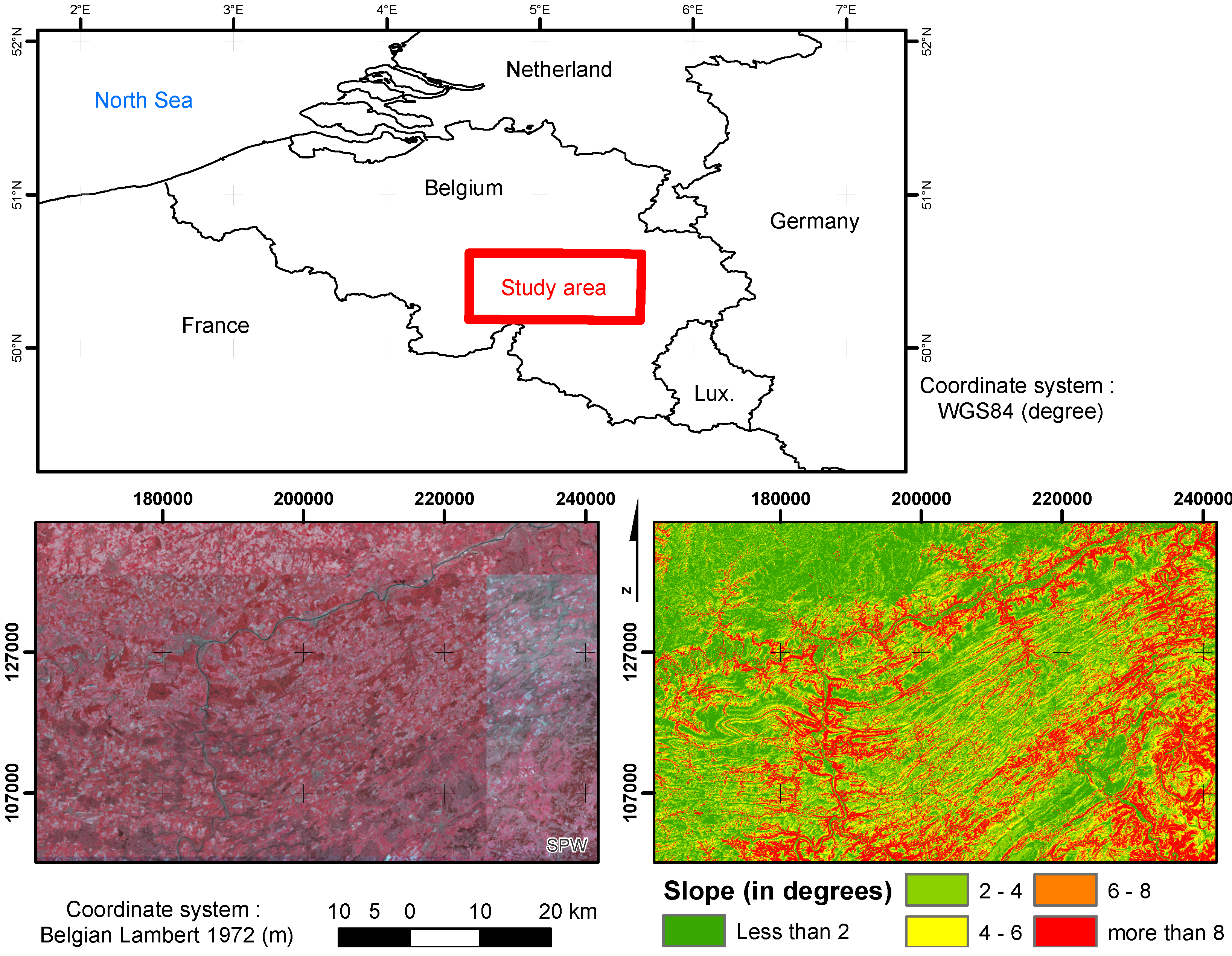
The study area is located in the Walloon region (Southern part of Belgium). This is a very fragmented landscape including coniferous forests (mainly spruce and other sempervirent species), deciduous broadleaved forests (mainly oaks and beeches), crop fields, natural and managed grasslands, peatlands, small water bodies, extraction areas as well as dense and sparse urban fabrics.
There are no mountainous terrains in Belgium, but a topography that is mainly driven by a dense hydrological network. In order to test our hypothesis, the experimental study focuses on the ravine maple stands, which grow on relatively steep slope and rocky soil. This biotope is particularly sparse, but at least present in five of the biogeographical regions of Wallonia. A rectangular study area (Figure 1) was delineated to include the majority of these biotopes present in Belgium. This region is relatively flat (slopes smaller than 7 percents) except in the valleys.
Two types of input data were available in the study area. First, a mosaic of ortho-rectified aerial photographs upscaled to 2 m resolution and including four spectral bands; Second, a LIDAR point cloud dataset rasterized at 2 m resolution.
The aerial photographs cover the entire study area. This coverage was done with several flights between March and April 2015. Image acquisition included four spectral bands (blue, green, red and near-infrared) at a spatial resolution of 0.25 m. The images available for the analysis were already ortho-rectified, mosaicked and rescaled in bytes. In order to avoid too much local heterogeneity, which would affect classification process, the original images were resampled at 2 m resolution using the mean values of all contributing pixels.
The LIDAR dataset was acquired in spring 2013 and 2014. The minimum sampling density is of 0.8 points per square meter. First and last returns were used to extract the ground elevation and the vegetation canopy height. In addition, this dataset required specific mathematical morphology analysis in order to remove some artifacts: a gray scale opening was applied in order to remove power lines. A digital elevation model (DEM) and a Digital Surface Model (DSM) of the vegetation were derived from the last and first returns, respectively. A Digital Height Model (DHM) was then obtained by subtracting the DEM from the DSM.
In addition to the remote sensing data, a vector database describing the biotopes inside Belgian protected areas from the European network of natural sites (NATURA2000) was available. This database was produced by the Walloon administration for Nature and Forest based on expert knowledge and exhaustive field inventories (all polygons). It is considered as the best available information about ravine forests in Wallonia and was therefore used as a reference. In order to ensure and improve the reliability of this map, polygons with visible clear cuts on the 2015 othophotos were manually removed from this reference.
3. Method
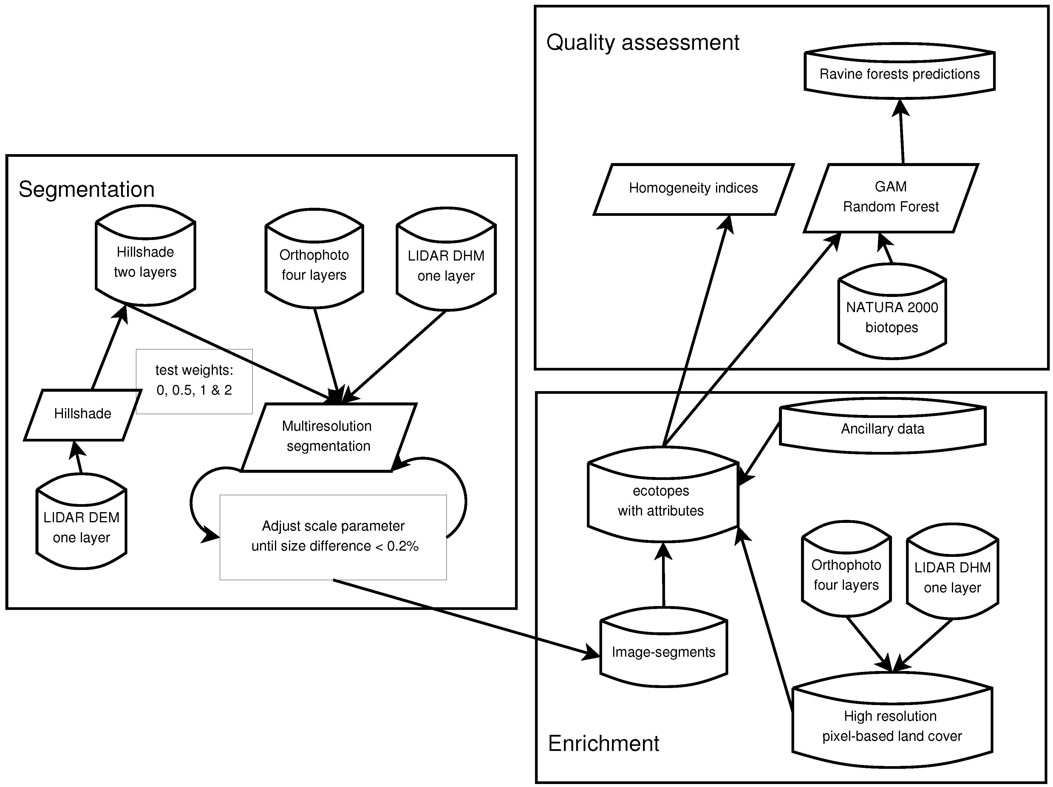
The core of the proposed process is the simultaneous segmentation of the topographic, spectral and height information. The resulting image segments are then enriched by computing a set of attributes based on remote sensing and ancillary data. The potential of the proposed method to automatically delineate meaningful spatial regions is assessed based on two expected properties of the ecotopes: a large homogeneity and the ability to build high performance ecological models. These steps are summarized on Figure 2.
3.1. Automated Ecotope Delineation
The three variables of interest to discriminate ecological function at the scale of the analysis are the land cover, the topography and the soil type. However, the available soil type information was not precise enough and could be partly inferred by the topography. We therefore focused on variables that could be directly inferred by remote sensing: topography and land cover.
The multiresolution segmentation algorithm [34] was used to automatically delineate ecotopes. This algorithm can be tuned by a set of four parameters: the scale, the weight of the raster layer, the shape and the compactness. The scale parameter defines the maximum acceptable value of the change of heterogeneity when merging two neighboring image-segments. Increasing the scale parameter therefore increases the size of the image-segments. The weight of the layers defines how much each raster layer will contribute to the heterogeneity difference of the merged image-segments as shown in Equation (1):
where is the total heterogeneity difference after merging based on the raster layers, is the weight of each raster layer, is the heterogeneity of image-segments 1 and 2 for layer L; and are the number of pixels in image-segments 1 and 2; and are the heterogeneity indices of image-segments 1 and 2. Then, the shape parameter defines the proportion of the heterogeneity index that is based on the shape of the image-segment. Increasing the shape parameter therefore reduces the contribution of a large heterogeneity difference after merging the image-segment. The compactness parameter determines if this shape index should favor compact image-segments (similar to a disk) or smooth image-segments (similar to a rectangle).
The efficiency of a segmentation combining LIDAR height and multispectral image had already been proven [26]. Our working hypothesis is that simultaneously combining the topographic information with the spectral values of the orthophotos and the DHM derived from the LIDAR would improve the delineation of the ecotopes. The segmentation results are therefore compared with different weights to the topographic information with respect to the other layers. For the sake of a fair comparison, the average size of the image-segments is fixed to approximately 2 ha (Two hectare on average corresponds to smallest ecological management units according to a group of users including biodiversity researchers and managers.) To do so, the composite image was first segmented with a scale parameter of 50, a shape parameter of and a compactness of . The shape parameter was then reduced to and a larger scale parameter was obtained using binary search algorithm with a tolerance of on the total number of polygons obtained on the reference image segmentation (that is 318,380). Apart from the size that was fixed after the first segmentation, no other optimization of the segmentation was performed. The only difference between the segmentation is therefore the weight of the topographic component that is being tested with values of zero (only spectral and structural information), 0.5, 1 and 2 (increasing the influence of topographic information).
Including topography in segmentation required a transformation of the DEM data to highlight the different slope types and identify breaks. Because the segmentation algorithm is based on the minimization of the variance inside each image-segment, using DEM values would indeed tend to create many linear spatial regions along contour lines in areas of steep slopes, even if the slope is constant. Previous studies used the slope together with some curvature indices [18]. This is interesting for pedomorphic mapping, but (i) it then relies on arbitrary window size to compute minimum and maximum curvature and (ii) both sides of ridge and valley lines are in the same segment despites different sun illumination. In the case of ecotopes, the slope and the aspect of the slope are therefore more closely related to the functionnal homogeneity However, slope aspect could not be used by the segmentation algorithm because (i) it is undefined when the slope is null and (ii) it is a circular metric that jumps from 360 degrees to 0 degree for the same azimuthal direction. For those reasons, Janowski et al. [27] used easting and northing instead of azimuth. For the ecotopes, two synthetic hillshade maps were derived along the North-South and the East-West transects using Equation (2), because this is the variable that is the most directly linked with the potential solar energy.
where and are the hypothetical sun zenithal and azimuthal angles, respectively, and and are derived from the DEM using a 3-by-3 moving window. The use of 3-by-3 windows corresponds to local hillshade at a high spatial resolution (2 m), so that only pixels with similar hillshade values are likely grouped together by the segmentation algorithm. The shape parameter of that is used in the segmentation process aims at preserving the compacity of the image segment when isolated pixels have a markedly different orientations than their surroundings, but image-segments are expected not to merge when there is a change of slope.
In practice, synthetic hillshade maps were created by setting a large sun zenith angle (75°) for four sun azimuth angles (0°, 90°, 180°, 270°). The difference between the results of both pairs of opposite theoretical sun azimuth angles were then computed. Cast shadows were ignored in this process because the aim of the hillshade is only to provide a continuous topographic characterization. As can be seen on Figure 3, the values of the hillshade are equal on flat surfaces and on slopes oriented with 45° or 135° azimuths. In the case of flat areas, the value in two opposite directions is indeed equal, so that their difference is zero for all azimuths. In the other case, the values are either positive or negative and they are equal for the orthogonal direction because 45° is the bisector of those azimuthal angles.
3.2. Quality Assessment
For the sake of ecological models, image-segments are enriched based on the proportion of land cover features that they contain as well as various soil and contextual attributes [16]. With all attributes being derived from external databases, the quality assessment focuses on the homogeneity of the image-segments (which is a key feature for ecotopes) (Section 3.2.2) and the ability to run performant ecological models (Section 3.2.3).
Due to the lack of other up-to-date high resolution land cover map of the Walloon region at the time of the study, a high resolution pixel-based land cover map was produced in order to characterize the ecotopes and build some of their homogeneity indices. While the production of this high resolution land cover database is out of the scope of this paper, it is briefly described in Section 3.2.1.
3.2.1. High Resolution Pixel-Based Land Cover
A Bayesian classifier with automated training sample extraction method [35] was used to classify 8 land cover types: bare soil, artificial, grassland, crops, coniferous, broadleaved, water and shrubs. The input image was based on the same datasets as the segmentation: the 4 spectral bands of the aerial photograph and the height information extracted from LIDAR. The a priori probability was computed based on the frequency of each land cover type within two height classes (below and above 50 cm). Because of the high reliability of the LIDAR DHM, this step was particularly useful to discriminate forests, shrubs and buildings from the other land covers. The training dataset was compiled based on existing datasets covering the study area, including a 2007 land cover map from the Walloon Region, Open Street Map data [36] and forest inventory data from the Nature and Forest Department. The results were then consolidated with a crop mask in order to discriminate grassland and cropland. Furthermore, the classification of forest types was consolidated in the homogeneous region thanks to a classification of Sentinel-2 cloud-free images of early spring and mid summer 2016 (assuming that the forest type does not change from year to year and excluding clear cuts from the analysis).
For the validation, a simple random sample of 700 points was photointerpreted on the orthophoto with a geolocation tolerance of 5 m and ambiguous points were verified on the ground. The estimated overall accuracy of the consolidated product ( with a confidence) was above the other products, therefore it was considered as our best reference in the frame of this paper.
3.2.2. Homogeneity Measures
In order to test the hypothesis of this study, different homogeneity indices have been computed. Those indices look at the homogeneity from land cover (based on the high resolution land cover layer), from the topography and from the soil types. They are compared with an arbitrary regular grid with the same cell area than the average polygon size, which provides a reference considering the segmentation ratio. Because of the specific interest towards a biotope that is mainly present in areas of steep slopes, the homogeneity indices were not only computed for all the study area, but also for a subset composed of the polygons with an average slope above 10 degrees.
Giving more weight to the topographic bands could affect the homogeneity in terms of land cover delineation. In order to control a potential loss of land cover homogeneity, the average purity level was computed for each segmentation. The proportion of each land cover class was computed inside each polygon based on the high-resolution pixel-based land cover classification presented in Section 3.2.1. The purity index is then defined as the average of the maximum values of land cover proportions of each image-segment.
From the topographic point of view, the primary variable of interest is the slope. The slope was measured on a smoothed version of the 2 m DEM in order to remove micro-topography effects and to remove artifacts due to the noise of the dataset. Because the slope is a quantitative variable, its heterogeneity was estimated using the standard deviation (STD) inside each polygon. For the aspect of the slope, standard deviation could not be used because of the break between 0 and 360°. The azimuth values were therefore converted into nine categories, including in eight directions (North, North-East, East, South-East, South, South-West, West and North-West) plus one class for the flat areas (where the aspect is undefined). The purity index of these nine categories is then computed like in the case of the land cover.
Finally, an independent data source was also considered: the soil map. The purity index for soil drainage classes and soil depth classes was used as an additional indirect indicator of the polygon homogeneity. Those two soil classes were derived from the digital soil map of the Walloon region. The precision of this map corresponds to a scale of 1/25,000, which is coarser than the polygons delineation, but this uncertainty affects all polygon boundaries in a similar way.
3.2.3. Biotope Models
In addition to the homogeneity measures, a fitness to purpose analysis was implemented. The sensitivity of two state-of-the-art algorithms, namely Random Forest (RF) and Generalized Additive Model (GAM), has been tested for the detection of ravine maple forests. Each model was calibrated using the same workflow for each of the segmentation results.
First, a large set of attributes have been derived from existing database and GIS analysis. This set includes bioclimatic variables interpolated from Worldclim [37], soil variables, topographic variables and land cover variables obtained by zonal statistics within each ecotope. Those variables have been selected based on expert knowledge and their contribution to habitat suitability models have been assessed in a previous study [16].
Calibration and validation polygons were then selected by crossing the ecotope database with the polygons of the NATURA 2000 database. An ecotope was labeled as a ravine maple forest biotope if more than half of its area was covered by its equivalent in the Natura 2000 cartography. To obtain a presence/absence dataset, ecotopes matching with ravine maple forests were considered as presence, while ecotopes matching with any other forest biotope were considered as an absence.
Different quality indices were used to validate the model, including the Overall Accuracy (OA) and the Area Under the Curve (AUC) of the model as well as producer and user accuracy (PA and UA) of the optimal binary classification between ravine forest and other forest biotope. In order to evaluate the accuracy of the model to detect ravine forests among all other biotopes, another overall accuracy was calculated taking into account all surfaces covered by Natura 2000 surveys (OA_Tot). Those indices were computed for the validation polygons which have been separated from the rest of the dataset before the calibration step. In order to provide an unbiased estimate of the correctly classified areas, the ecotope polygons were used as sampling units and their areas were taken into account [38]. The optimal binary classification was automatically determined based on the best compromise between sensitivity and specificity.
4. Results
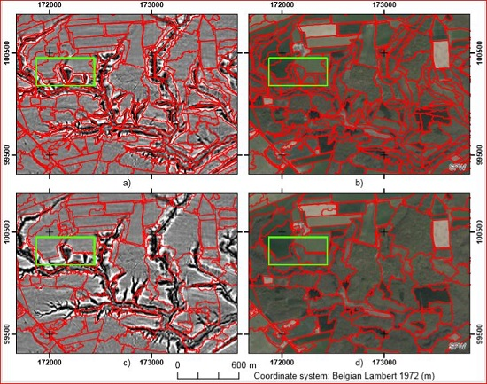
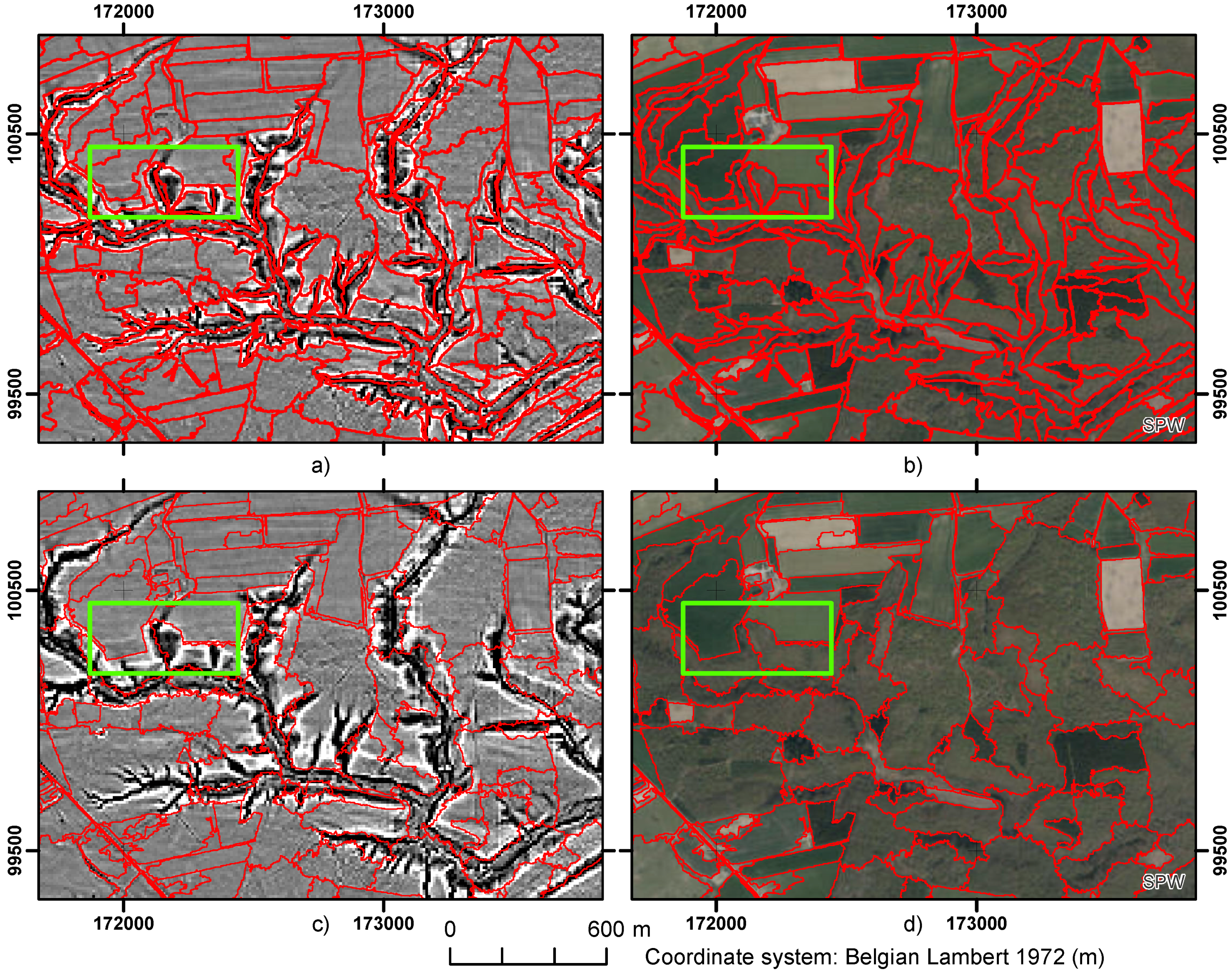
By design, approximately 318400 image-segments were automatically created in the study area (with a range of 500 polygons, that is less than 0.2 percent). A visual check did not catch any macroscopic errors, but revealed most of the topographic features hidden by the vegetation on the aerial image. Figure 4 shows a subset of the segmentation result, highlighting the impact of the topography on the image-segments created inside patches of homogeneous land cover. As expected, areas of homogeneous slope are well delineated in addition to the land cover induced partitioning. Furthermore, the limits of the ecotopes are consistent with the pattern of slope curvature, which were not used for the segmentation.
Quantitative results related to the homogeneity of the image-segments are summarized in Table 1 and Table 2. Overall, the advantage of automatically partitioned landscape against a regular grid of the same size is obvious. The results indeed show that the heterogeneity of the topographic attributes decreases and the separability of ecotopes increases when the partition of the landscape is determined by topography and land cover. As shown in Figure Table 2, the results within the subset of polygons with a slope above 15 percent further highlight the differences where the terrain plays a bigger role in the definition of the polygons.
The analysis of the predictive model indicate that the ecotopes are appropriate mapping units to map ravine forest in the study area. The overall accuracy of the best model is indeed (Table 3). However, this value does not completely reflect the errors of the model because ravine forests are rare in the study area and specific to the polygons with a majority of broadleaved trees. Additional indices measured on a subset of the ecotopes with a majority of broadleaved trees are therefore more relevant to compare the different scenarios. On this subset, the use of topographic information to delineate polygons had a significantly positive impact on the results of the models. This confirms the results obtained by homogeneity measures (Table 1 and Table 2). However, the best prediction is achieved for the GAM model when the weight of the topographic information is equal to the weight of the spectral information and the performances of the model decrease with the weight of 2.
The number of matching polygons increases when the segmentation uses more topographic components (Table 3). This is due to the fact that the polygon boundaries match the Natura 2000 boundaries closer than in the case without topographic contributions, but also because the polygons become on average smaller in rugged terrain when the topography is taken into account, as shown in Table 2.
5. Discussion
This study demonstrates that automated image segmentation simultaneously combining topographic information from LIDAR with the spectral information from optical sensors provides ecologically relevant polygons. Two facets of the results are discussed in this section: the technical quality of the results and the usefulness of the model for biodiversity studies.
5.1. Consistency of the Polygons
The objective of this paper was to build homogeneous polygons that would better match the concept of ecotopes than a delineation solely accounting for the land cover. While it was foreseen that the addition of topographic information to the segmentation process would reduce the topographic heterogeneity, the increased land cover homogeneity was surprising. This could be due to the long term land management practices that optimized land use based on the topography (for example, most crop fields are located on flat areas while steep slope are mainly covered by forests). Such patterns have been observed in the landscape, but the causality should be further investigated.
The results of the model shows that including topographic information improves the correspondence between ecotopes polygons and the field mapping of ravine forest biotope. The increased number of matches is partly due to the reduction of the average polygon size inside rugged terrain (about for the weight of 2). The reduction of the size is however not sufficient to explain the large increase in the number of matches. This could be better explained by the fact that presence of biotope is highly dependent on the topographic situation. Indeed, contrasted situations such as south or north hillside leads to very different abiotic features. Furthermore, even a small difference of slope leads to different water intakes leading also to different vegetation communities.
Even if the model weren’t created in the best conditions due to the scarcity of the biotope, we can stress that we see a large leap in the AUC of the models (more than for both RF and GAM) by adding topographic data in the segmentation process. Concerning the model accuracy, the big increase observed by adding topographic data is consistent with the improvement observed by the heterogeneity indices. However, we can see that the indices of the models don’t follow the same trend than the heterogeneity indices and are less correlated with the level of contribution of topographic data. This is probably due to the fact that we model a rare biotope with scarce presence data. Thus, the overall quality of the models is sensitive to the polygons selected in the calibration/validation process.
In this study, the average size was selected according to user requirements and fixed in order to fairly compare the contributions of the models. However, the size could also be optimized based on data driven features [39,40] In this case, the weight of the topography, the vegetation height and the spectral values of the images should be considered to determine an optimal size. However, the observed difference between the trend in terms of ecotope purity and the trend of the fitness-to-purpose analysis should be further investigated as a potential issue to the use of a single optimization criteria.
On the other hand, landscape and landform analysis very much depends on the scale of the process being addressed and a hierarchical approach could help to extract additional characteristics from the landscape. For instance, elevation and curvature are important features at coarser scale to identify ridges or valleys. However, ridges and valley landforms include two sides facing opposite directions, which is not homogeneous in terms of insulation. The use of hillshade at local scale obviously placed the emphasis on potential insulation, but it also split image-segments in places of strong positive or negative curvature, which contributed to the improvement of characteristic soil properties. Identifying pattern from another scales could however be necessary to cover the processes that occur in more mountainous areas.
5.2. Usefulness of Biotope Models
The high (above for both GAM and RF) AUC of the best models shows that models based on ecotope polygons are very consistent. However, despite the high specificity and sensitivity of the models, the user accuracy of the ravine forest class is very low. This low user accuracy can be explained by three different factors.
First, the ravine forests are rare in the study area. As a result, even a very small proportion of false positive had a strong impact on the user accuracy. Nevertheless, the absolute number of forest remains small, so that the models could help field prospecting by narrowing the search area to fewer than five percents of the total surface of forests.
Second, the models were used to test a concept and compare different segmentation strategies, but they could be tuned for other specific purposes. The selected optimization criteria, based on the sensitivity and the specificity, favored a solution that maximized the sensitivity because the specificity computed on a large proportion of absences was rapidly very high (above ), then slowly increased. This type of optimization is particularly useful for restraining the surveyed area in order to exhaustively map a specific biotope. Another threshold for binary classification could seek an optimum between producer’s and user’s accuracy based on the F-Score. With this alternative, the UA would be 0.63 and the PA would be 0.65, which is a good compromise for a generic result but less interesting for the identification of unknown biotopes of high biological interest.
Third, the model is limited by the available data, which does not replace field based observations. For instance, typical ferns in the understory are not visible by remote sensing. On the other hand, the ecotope might include all conditions for the development of maple ravine forests, but a different type of forest could have developed because of historical land management of the ecotope. From this point of view, a substantial proportion of the false positives could be considered priority zones for biotope restoration.
Nevertheless, values of user accuracy that we are discussing about are dependent of the correctly classified ravine forest among other broadleaved forests.If we take a look at total overall accuracy values, they show an excellent prediction of ravine forest in our study area therefore moderating the poor user accuracy previously discussed.
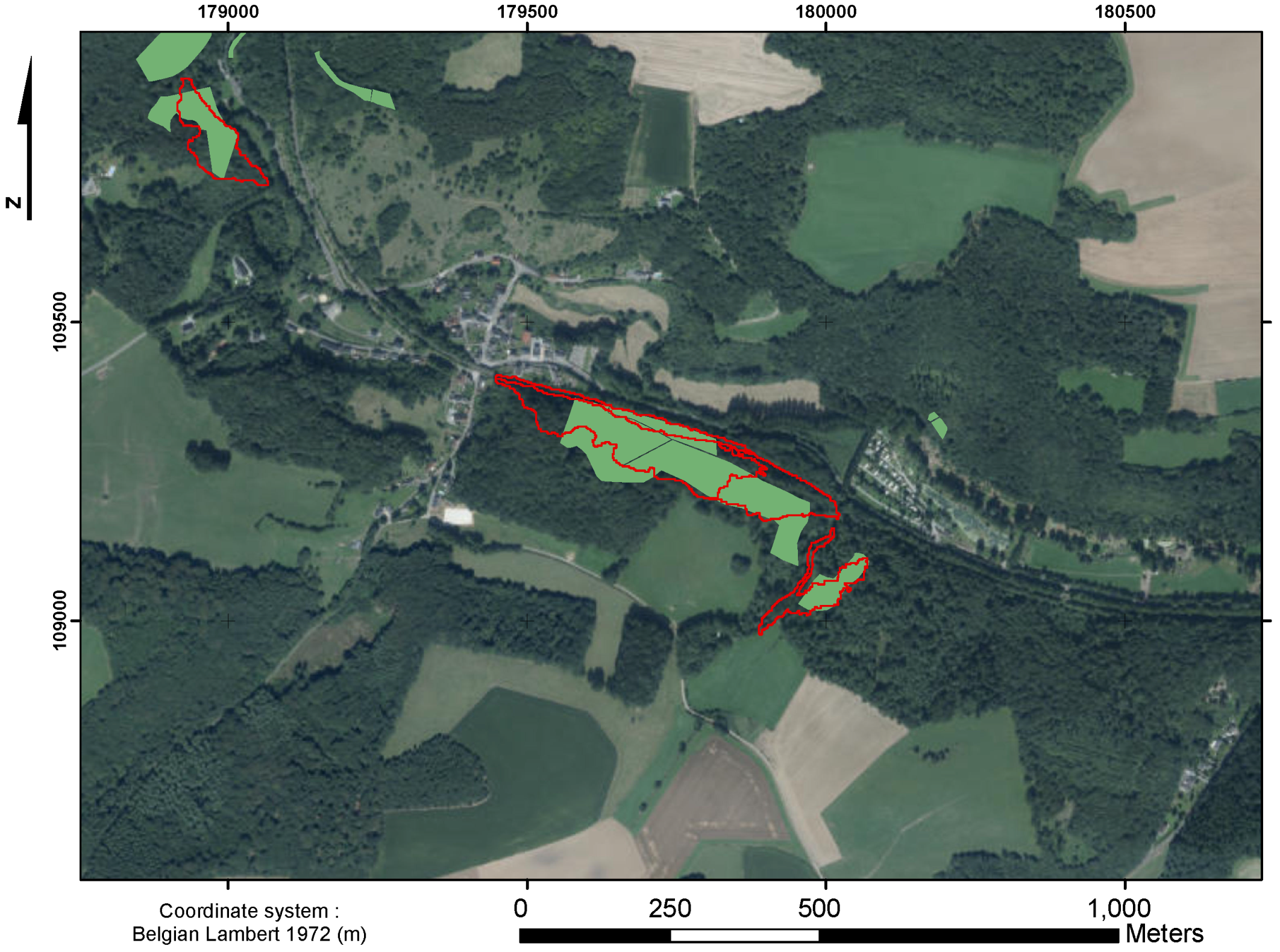
Referring to the field data, forest communities don’t follow a logic of tangible frontier, but they look like a gradient of vegetation communities mixing with another one. Limits are vague, but the conceptual model of the geographic database uses crisp boundaries to represent those transition areas. This conceptual mapping model into the so-called spatial regions is not specific to the GEOBIA, but it is also performed on the field when a boundary has to be drawn. While about half of the boundaries are matching the boundaries of the reference polygons with precision close to 10 m, diverging delineation occurs on the other half of the boundaries (Example on Figure 5). An independent field campaign was unable to undoubtedly and consistently arbitrate between the two datasets. Despite its limitations, the repeatability of the automated image segmentation makes it very useful in prospective studies or to guide interpretation on the field. However, the use of sharp boundaries could be an issue to represent gradients of vegetation or to be associated with punctual observations. It is therefore of paramount importance to remember that the proposed mapping strategy is a model used to represent the landscape in a way that closely matches the definition of biotopes from the field, but that there is no universal representation of nature.
6. Conclusions
This study demonstrates that hillshade layers can be used simultaneously with spectral information to improve the automated delineation of ecotopes in a GEOBIA framework. The AUC of predictive ecological models was improved by when the ecotopes were delineatd using these topographic layers. Furthermore, the inclusion of topographic features in the segmentation process also improved the purity in terms of land cover, probably due to the indirect impact of the topography on the land use in the study area.
The good results at small scale factor suggests that the proposed GEOBIA workflow could be tested at larger scale factor in combination with curvature indices in order to generate homogeneous landforms with minimal arbitrary decisions.
Author Contributions
Conceptualization, J.R., A.B., W.C., M.D. and P.D.; Formal analysis, J.R. and A.B.; Methodology, J.R., A.B. and W.C.; Supervision, M.D. and P.D.; Validation, J.R. and A.B.; Writing—original draft, J.R., A.B. and W.C.; Writing—review and editing, J.R., A.B., M.D. and P.D.
Funding
This research was funded by Fédération Wallonie-Bruxelles in the frame of the Lifewatch-WB project.
Acknowledgments
The authors thank the three reviewers for their constructive comments.
Conflicts of Interest
The authors declare no conflict of interest.
Dataset
Extended database is available on http://maps.elie.ucl.ac.be/lifewatch/ecotopes.html.
Abbreviations
The following abbreviations are used in this manuscript:
| AUC | Area Under the curve |
| DEM | Digital Elevation Model |
| DHM | Digital Height Model |
| GAM | Generalized Additive Model |
| GEOBIA | Geographic Object-Based Image Analysis |
| PA | Producer’s accuracy |
| OA | Overall accuracy |
| RF | Random Forest |
| STD | Standard Deviation |
| UA | User’s accuracy |
References
- Mittermeier, R.A.; Turner, W.R.; Larsen, F.W.; Brooks, T.M.; Gascon, C. Global Biodiversity Conservation: The Critical Role of Hotspots. In Biodiversity Hotspots: Distribution and Protection of Conservation Priority Areas; Zachos, F.E., Habel, J.C., Eds.; Springer: Berlin/Heidelberg, Germany, 2011; pp. 3–22. [Google Scholar]
- Myers, N.; Mittermeier, R.A.; Mittermeier, C.G.; da Fonseca, G.A.B.; Kent, J. Biodiversity hotspots for conservation priorities. Nature 2000, 403, 853–858. [Google Scholar] [CrossRef] [PubMed]
- Ostermann, O.P. The need for management of nature conservation sites designated under Natura 2000. J. Appl. Ecol. 1998, 35, 968–973. [Google Scholar] [CrossRef]
- Loidi, J. Preserving biodiversity in the European Union: The Habitats Directive and its application in Spain. Plant Biosyst. 1999, 133, 99–106. [Google Scholar] [CrossRef]
- Wells, M.; Timmer, F.; Carr, A. Understanding Drivers and Setting Targets for Biodiversity in Urban Green Design. In Green Design: From Theory to Practice; Yeang, K., Spector, A., Eds.; Black Dog Publishing: London, UK, 2011. [Google Scholar]
- Donald, P.F.; Evans, A.D. Habitat connectivity and matrix restoration: The wider implications of agri-environment schemes. J. Appl. Ecol. 2006, 43, 209–218. [Google Scholar] [CrossRef]
- Bryn, A. Recent forest limit changes in south-east Norway: Effects of climate change or regrowth after abandoned utilisation? Norsk Geogr. Tidsskr.-Nor. J. Geogr. 2008, 62, 251–270. [Google Scholar] [CrossRef] [Green Version]
- Bunce, R.; Metzger, M.; Jongman, R.; Brandt, J.; De Blust, G.; Elena-Rossello, R.; Groom, G.B.; Halada, L.; Hofer, G.; Howard, D.; et al. A standardized procedure for surveillance and monitoring European habitats and provision of spatial data. Landsc. Ecol. 2008, 23, 11–25. [Google Scholar] [CrossRef]
- Pokharel, B.; Dech, J.P. An ecological land classification approach to modeling the production of forest biomass. For. Chron. 2011, 87, 23–32. [Google Scholar] [CrossRef] [Green Version]
- Maes, J.; Egoh, B.; Willemen, L.; Liquete, C.; Vihervaara, P.; Schägner, J.P.; Grizzetti, B.; Drakou, E.G.; La Notte, A.; Zulian, G.; et al. Mapping ecosystem services for policy support and decision making in the European Union. Ecosyst. Serv. 2012, 1, 31–39. [Google Scholar] [CrossRef] [Green Version]
- Egoh, B.; Drakou, E.G.; Dunbar, M.B.; Maes, J.; Willemen, L. Indicators for Mapping Ecosystem Services: A Review; European Commission, Joint Research Centre (JRC): Ispra, Italy, 2012. [Google Scholar]
- Spanhove, T.; Borre, J.V.; Delalieux, S.; Haest, B.; Paelinckx, D. Can remote sensing estimate fine-scale quality indicators of natural habitats? Ecol. Indic. 2012, 18, 403–412. [Google Scholar] [CrossRef]
- Borre, J.V.; Paelinckx, D.; Mücher, C.A.; Kooistra, L.; Haest, B.; De Blust, G.; Schmidt, A.M. Integrating remote sensing in Natura 2000 habitat monitoring: Prospects on the way forward. J. Nat. Conserv. 2011, 19, 116–125. [Google Scholar] [CrossRef]
- Guisan, A.; Zimmermann, N.E. Predictive habitat distribution models in ecology. Ecol. Model. 2000, 135, 147–186. [Google Scholar] [CrossRef]
- Osborne, P.E.; Alonso, J.; Bryant, R. Modelling landscape-scale habitat use using GIS and remote sensing: A case study with great bustards. J. Appl. Ecol. 2001, 38, 458–471. [Google Scholar] [CrossRef]
- Delangre, J.; Radoux, J.; Dufrêne, M. Landscape delineation strategy and size of mapping units impact the performance of habitat suitability models. Ecol. Inform. 2017, 47, 55–60. [Google Scholar] [CrossRef]
- Ellis, E.C.; Wang, H.; Xiao, H.S.; Peng, K.; Liu, X.P.; Li, S.C.; Ouyang, H.; Cheng, X.; Yang, L.Z. Measuring long-term ecological changes in densely populated landscapes using current and historical high resolution imagery. Remote Sens. Environ. 2006, 100, 457–473. [Google Scholar] [CrossRef]
- Gerçek, D. A Conceptual Model for Delineating Land Management Units (LMUs) Using Geographical Object-Based Image Analysis. ISPRS Int. J. Geo-Inf. 2017, 6, 170. [Google Scholar] [CrossRef]
- Chan, J.C.W.; Paelinckx, D. Evaluation of Random Forest and Adaboost tree-based ensemble classification and spectral band selection for ecotope mapping using airborne hyperspectral imagery. Remote Sens. Environ. 2008, 112, 2999–3011. [Google Scholar] [CrossRef]
- Haber, W. Basic concepts of landscape ecology and their application in land management. Physiol. Ecol. Jpn. 1990, 27, 131–146. [Google Scholar]
- Haber, W. Using landscape ecology in planning and management. In Changing Landscapes: An Ecological Perspective; Springer: Berlin, Germany, 1990; pp. 217–232. [Google Scholar]
- Hong, S.K.; Kim, S.; Cho, K.H.; Kim, J.E.; Kang, S.; Lee, D. Ecotope mapping for landscape ecological assessment of habitat and ecosystem. Ecol. Res. 2004, 19, 131–139. [Google Scholar] [CrossRef]
- Shen, L.; Wu, L.; Dai, Y.; Qiao, W.; Wang, Y. Topic modelling for object-based unsupervised classification of VHR panchromatic satellite images based on multiscale image segmentation. Remote Sens. 2017, 9, 840. [Google Scholar] [CrossRef]
- Nemmaoui, A.; Aguilar, M.; Aguilar, F.; Novelli, A.; García Lorca, A. Greenhouse crop identification from multi-temporal multi-sensor satellite imagery using object-based approach: A case study from Almería (Spain). Remote Sens. 2018, 10, 1751. [Google Scholar] [CrossRef]
- Ruan, R.; Ren, L. Urban ecotope mapping using QuickBird imagery. In Proceedings of the IEEE International Geoscience and Remote Sensing Symposium, Barcelona, Spain, 23–28 July 2007; pp. 2963–2966. [Google Scholar]
- Geerling, G.; Vreeken-Buijs, M.; Jesse, P.; Ragas, A.; Smits, A. Mapping river floodplain ecotopes by segmentation of spectral (CASI) and structural (LiDAR) remote sensing data. River Res. Appl. 2009, 25, 795–813. [Google Scholar] [CrossRef]
- Janowski, L.; Trzcinska, K.; Tegowski, J.; Kruss, A.; Rucinska-Zjadacz, M.; Pocwiardowski, P. Nearshore Benthic Habitat Mapping Based on Multi-Frequency, Multibeam Echosounder Data Using a Combined Object-Based Approach: A Case Study from the Rowy Site in the Southern Baltic Sea. Remote Sens. 2018, 10, 1983. [Google Scholar] [CrossRef]
- Guilbert, E.; Moulin, B. Towards a common framework for the identification of landforms on terrain models. ISPRS Int. J. Geo-Inf. 2017, 6, 12. [Google Scholar] [CrossRef]
- Gerçek, D.; Toprak, V.; Strobl, J. Object-based classification of landforms based on their local geometry and geomorphometric context. Int. J. Geogr. Inf. Sci. 2011, 25, 1011–1023. [Google Scholar] [CrossRef]
- Drăguţ, L.; Eisank, C. Automated object-based classification of topography from SRTM data. Geomorphology 2012, 141, 21–33. [Google Scholar] [CrossRef] [PubMed] [Green Version]
- Gessler, P.; Chadwick, O.; Chamran, F.; Althouse, L.; Holmes, K. Modeling soil–landscape and ecosystem properties using terrain attributes. Soil Sci. Soc. Am. J. 2000, 64, 2046–2056. [Google Scholar] [CrossRef]
- Kravchenko, A.N.; Bullock, D.G. Correlation of corn and soybean grain yield with topography and soil properties. Agron. J. 2000, 92, 75–83. [Google Scholar] [CrossRef]
- Sternberg, M.; Shoshany, M. Influence of slope aspect on Mediterranean woody formations: Comparison of a semiarid and an arid site in Israel. Ecol. Res. 2001, 16, 335–345. [Google Scholar] [CrossRef]
- Baatz, M.; Schäpe, A. Multiresolution Segmentation—An optimization approach for high quality multi-scale image segmentation. In Angewandte Geographische Informationsverarbeitung XII; Strobl, J., Blaschke, T., Griesebner, G., Eds.; Wichmann-Verlag: Heidelberg, Germany, 2000; pp. 12–23. [Google Scholar]
- Radoux, J.; Bogaert, P. Accounting for the area of polygon sampling units for the prediction of primary accuracy assessment indices. Remote Sens. Environ. 2014, 142, 9–19. [Google Scholar] [CrossRef] [Green Version]
- OpenStreetMap Contributors. Planet Dump. 2017. Available online: https://www.openstreetmap.org (accessed on 24 September 2018).
- Hijmans, R.; Cameron, S.; Parra, J.; Jones, P.; Jarvis, A. Very high resolution interpolated climate surfaces for global land areas. Int. J. Climatol. 2005, 25, 1965–1978. [Google Scholar] [CrossRef] [Green Version]
- Radoux, J.; Bogaert, P. Good Practices for Object-Based Accuracy Assessment. Remote Sens. 2017, 9, 646. [Google Scholar] [CrossRef]
- Drăguţ, L.; Tiede, D.; Levick, S.R. ESP: A tool to estimate scale parameter for multiresolution image segmentation of remotely sensed data. Int. J. Geogr. Inf. Sci. 2010, 24, 859–871. [Google Scholar] [CrossRef]
- Radoux, J.; Defourny, P. Quality assessment of segmentation results devoted to object-based classification. In Object-Based Image Analysis; Springer: Berlin, Germany, 2008; pp. 257–271. [Google Scholar]
Figure 1.
Aerial orthophoto (left) and slope derived from the LIDAR images (right) on the study area.
Figure 1.
Aerial orthophoto (left) and slope derived from the LIDAR images (right) on the study area.

Figure 2.
Overall flowchart of the proposed method.

Figure 3.
False color composite of the hillshades along the North-South and East-West directions (left) and slope derived from the LIDAR images (right) on a subset of the study area. Shades of grey indicate that the hillshade values in the two orthogonal directions are equal while colored areas highlight the differences between the two directions.

Figure 4.
Image-segment boundaries (in red) overlaid on the curvature of the DEM at 10 m resolution (left) and the orthophoto from the Walloon Region (right, copyright SPW 2015). The images at the top (a,b) display the segmentation with the topographic bands (weight of 1); the images at the bottom (c,d) display the segmentation without the topographic bands. The green rectangle highlights an area where the land use boundaries follow the topography.

Figure 5.
Divergences of delineation of ravine forest in the Natura 2000 database (green polygons) and the automated segmentation (red outlines).
Figure 5.
Divergences of delineation of ravine forest in the Natura 2000 database (green polygons) and the automated segmentation (red outlines).


Table 1.
Homogeneity of the image-segment as a function of the segmentation weights. The grid is composed of squares with the same area as the average of image-segments. Large purity values and low average variance of the slope indicate a good segmentation.
Table 1.
Homogeneity of the image-segment as a function of the segmentation weights. The grid is composed of squares with the same area as the average of image-segments. Large purity values and low average variance of the slope indicate a good segmentation.
| 0 (No Topographic Layers) | 0.5 | 1 | 2 | Grid | |
|---|---|---|---|---|---|
| Slope variance | 4.21 | 4.00 | 3.90 | 3.83 | 4.82 |
| Aspect purity | 94.4 | 94.4 | 94.5 | 94.5 | 94.3 |
| Soil depth purity | 82.8 | 82.8 | 84.0 | 83.1 | 79.9 |
| Soil drainage purity | 80.1 | 80.9 | 81.3 | 81.7 | 80.4 |
| Land cover purity | 75.9 | 76.5 | 76.6 | 76.4 | 72.2 |
Table 2.
Homogeneity of the subset of image-segments with a slope greater than 15 percent. The grid is composed of squares with the same area as the average of image-segments. Large purity values and low average of slope variance indicate a good segmentation.
Table 2.
Homogeneity of the subset of image-segments with a slope greater than 15 percent. The grid is composed of squares with the same area as the average of image-segments. Large purity values and low average of slope variance indicate a good segmentation.
| 0 (No Topographic Layers) | 0.5 | 1 | 2 | Grid | |
|---|---|---|---|---|---|
| Slope variance | 10.6 | 8.1 | 7.1 | 6.2 | 11.6 |
| Aspect purity | 93.7 | 95.2 | 95.9 | 96.4 | 93.7 |
| Soil depth purity | 80.2 | 81.9 | 82.7 | 83.5 | 75.6 |
| Soil drainage purity | 79.7 | 81.8 | 82.4 | 82.5 | 78.3 |
| Land cover purity | 69.4 | 75.0 | 75.4 | 76.4 | 64.8 |
| Mean area (m2) | 20,466 | 17,379 | 16,432 | 15,577 | 19,016 |
Table 3.
Results of the different models of ravine forest predictions with respect to the weight of topography in the segmentation. Matches correspond to the number of ecotopes matching at more than 50 percent with biotopes survey polygons. The next rows show the different quality indices including the overall accuracy of ravine forest mapping in the study area (), the Overall Accuracy (OA), Area Under the Curve (AUC), Producer Accuracy (PA) and User Accuracy (UA) of the ravine forests for each model based on ecotopes covered by a majority of broadleaved trees.
| 0 | 0.5 | 1 | 2 | |
|---|---|---|---|---|
| Matches | 17 | 60 | 87 | 109 |
| RF | 99.7 | 99.8 | 99.8 | 99.7 |
| RF OA | 93.2 | 94.7 | 95.5 | 92.7 |
| RF AUC | 79.6 | 97.1 | 96.8 | 94.3 |
| RF PA | 77.9 | 97.0 | 95.3 | 92.7 |
| RF UA | 8.90 | 18.9 | 25.3 | 16.1 |
| GAM | 99.8 | 99.8 | 99.9 | 99.8 |
| GAM OA | 96.1 | 95.7 | 97.3 | 95.2 |
| GAM AUC | 81.4 | 95.6 | 97.6 | 95.2 |
| GAM PA | 77.2 | 93.1 | 97.0 | 92.7 |
| GAM UA | 15.0 | 21.9 | 37.2 | 22.5 |
© 2019 by the authors. Licensee MDPI, Basel, Switzerland. This article is an open access article distributed under the terms and conditions of the Creative Commons Attribution (CC BY) license (http://creativecommons.org/licenses/by/4.0/).
Share and Cite
MDPI and ACS Style
Radoux, J.; Bourdouxhe, A.; Coos, W.; Dufrêne, M.; Defourny, P. Improving Ecotope Segmentation by Combining Topographic and Spectral Data. Remote Sens. 2019, 11, 354. https://doi.org/10.3390/rs11030354
AMA Style
Radoux J, Bourdouxhe A, Coos W, Dufrêne M, Defourny P. Improving Ecotope Segmentation by Combining Topographic and Spectral Data. Remote Sensing. 2019; 11(3):354. https://doi.org/10.3390/rs11030354
Chicago/Turabian StyleRadoux, Julien, Axel Bourdouxhe, William Coos, Marc Dufrêne, and Pierre Defourny. 2019. "Improving Ecotope Segmentation by Combining Topographic and Spectral Data" Remote Sensing 11, no. 3: 354. https://doi.org/10.3390/rs11030354
Note that from the first issue of 2016, this journal uses article numbers instead of page numbers. See further details here.