
Improvement of Soil Moisture Retrieval from Hyperspectral VNIR-SWIR Data Using Clay Content Information: From Laboratory to Field Experiments


Abstract
:
1. Introduction
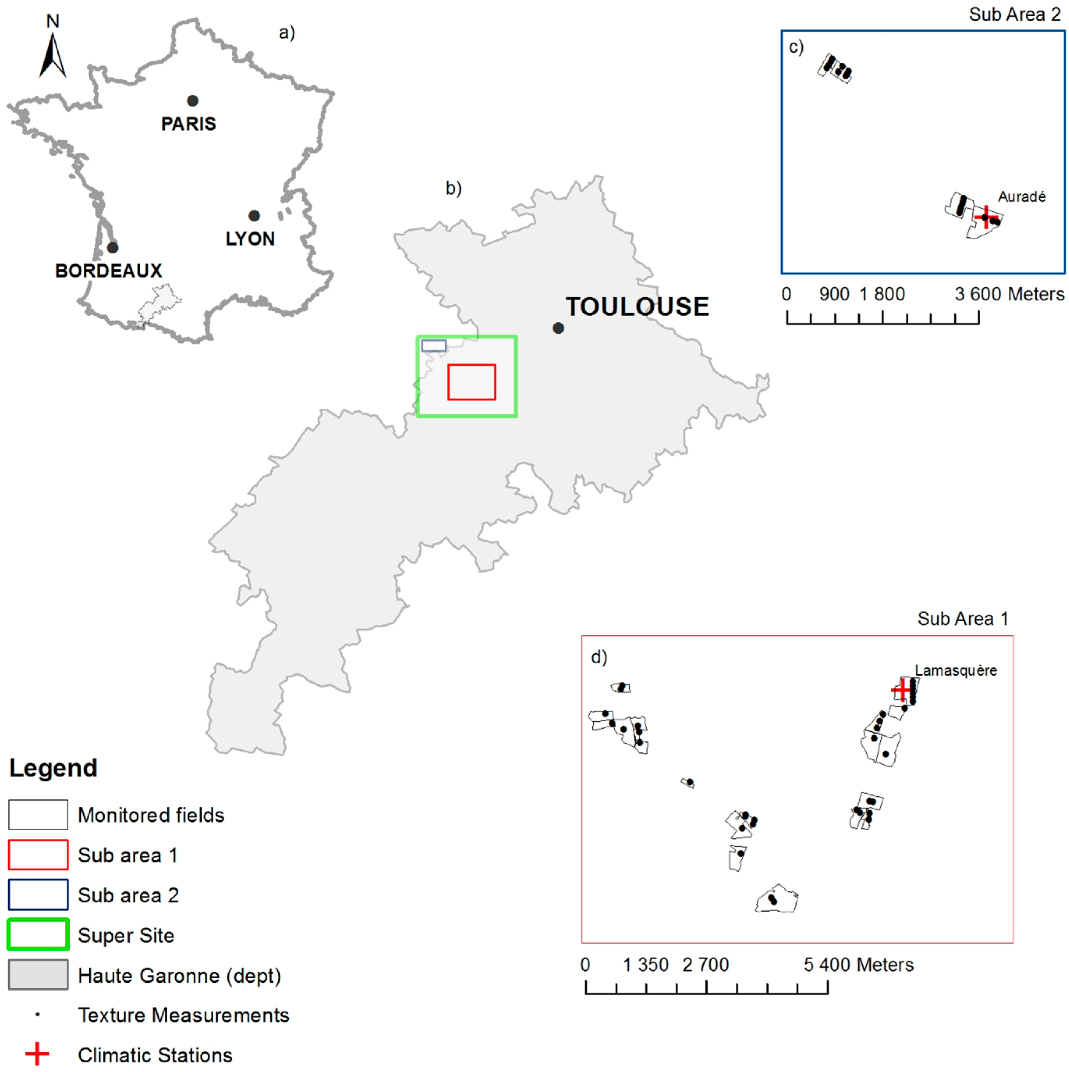
2. Study Site and Data Collection
2.1. Site Description

2.2. Soil Moisture Content
2.2.1. Laboratory Data
2.2.2. In-situ Data
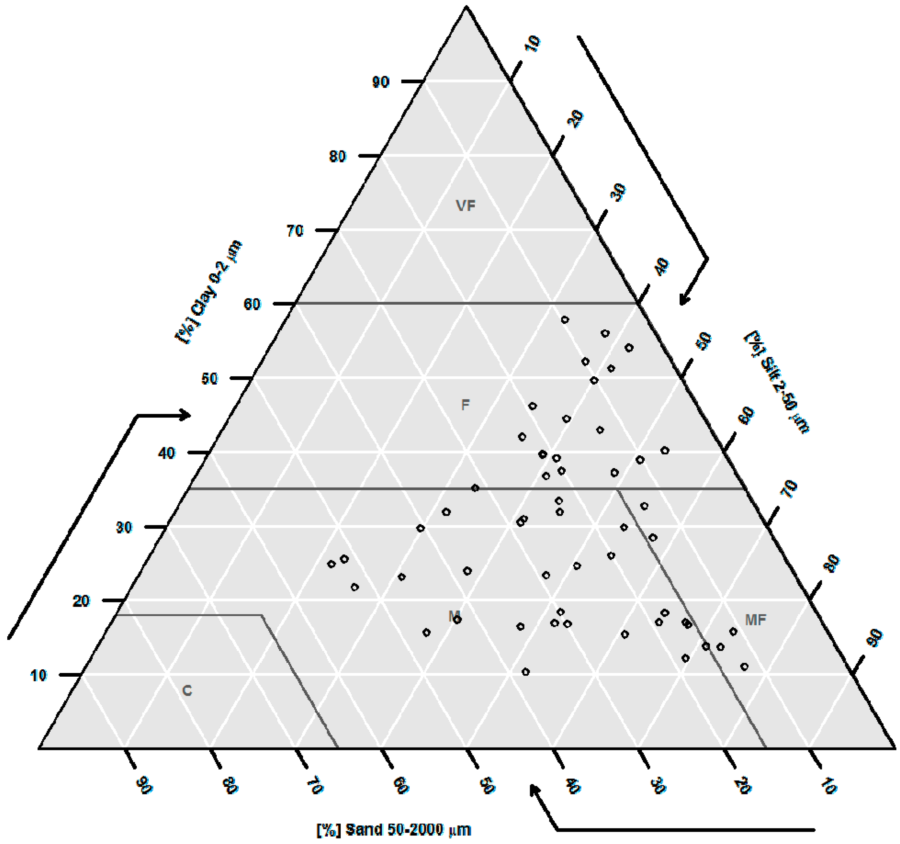
2.3. Clay Content

2.4. Spectral Signatures

| Spectral Range | Spectral Resolution | Spectral Sampling | |
|---|---|---|---|
| VNIR | 0.35–1.00 µm | 3 nm at 0.70 µm | 1.4 nm (0.35–1.05 µm) |
| SWIR | 1.00–2.50 µm | 10 nm at 1.40 µm | 2 nm (1.05–2.50 µm) |
| 12 nm at 2.10 µm |
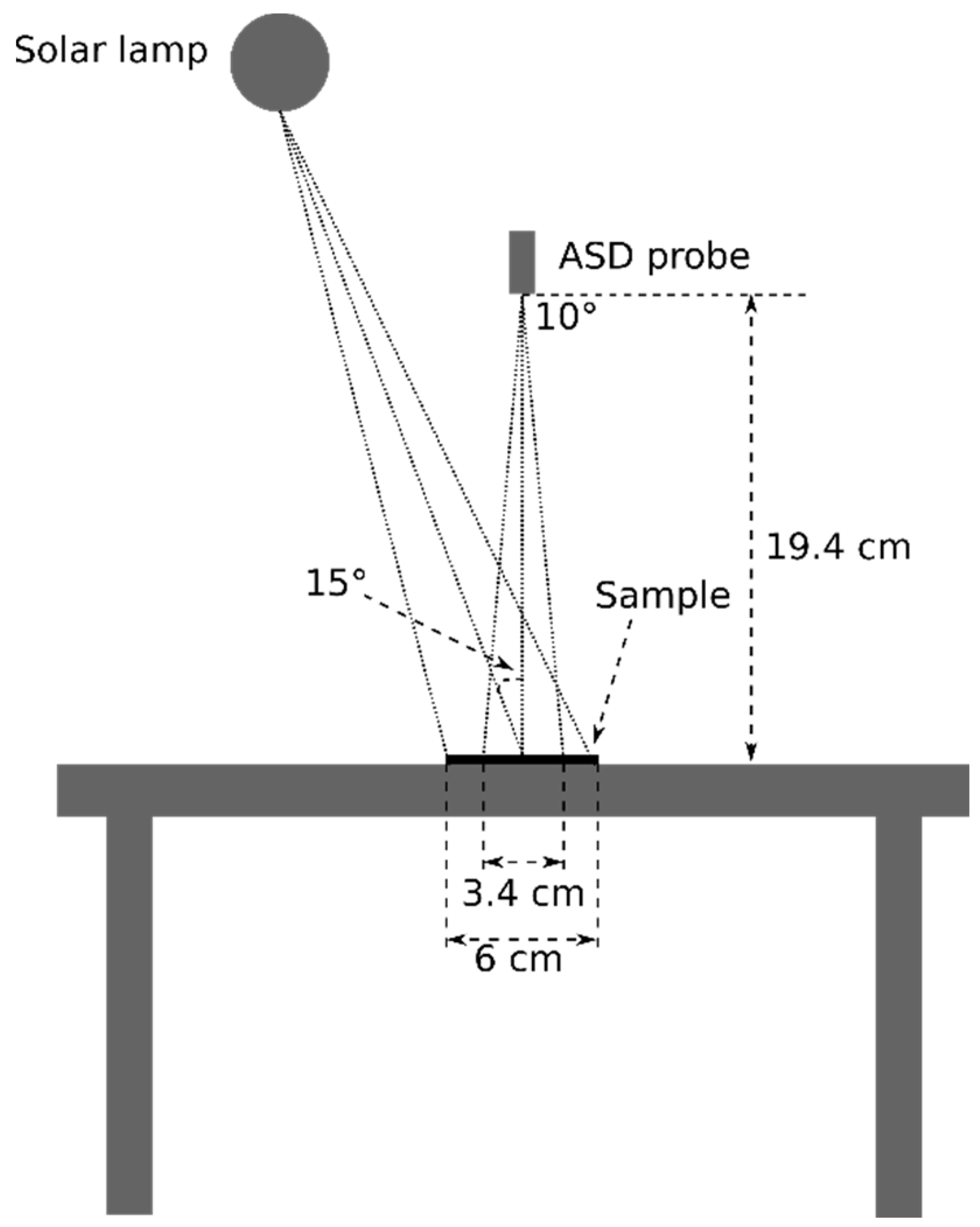
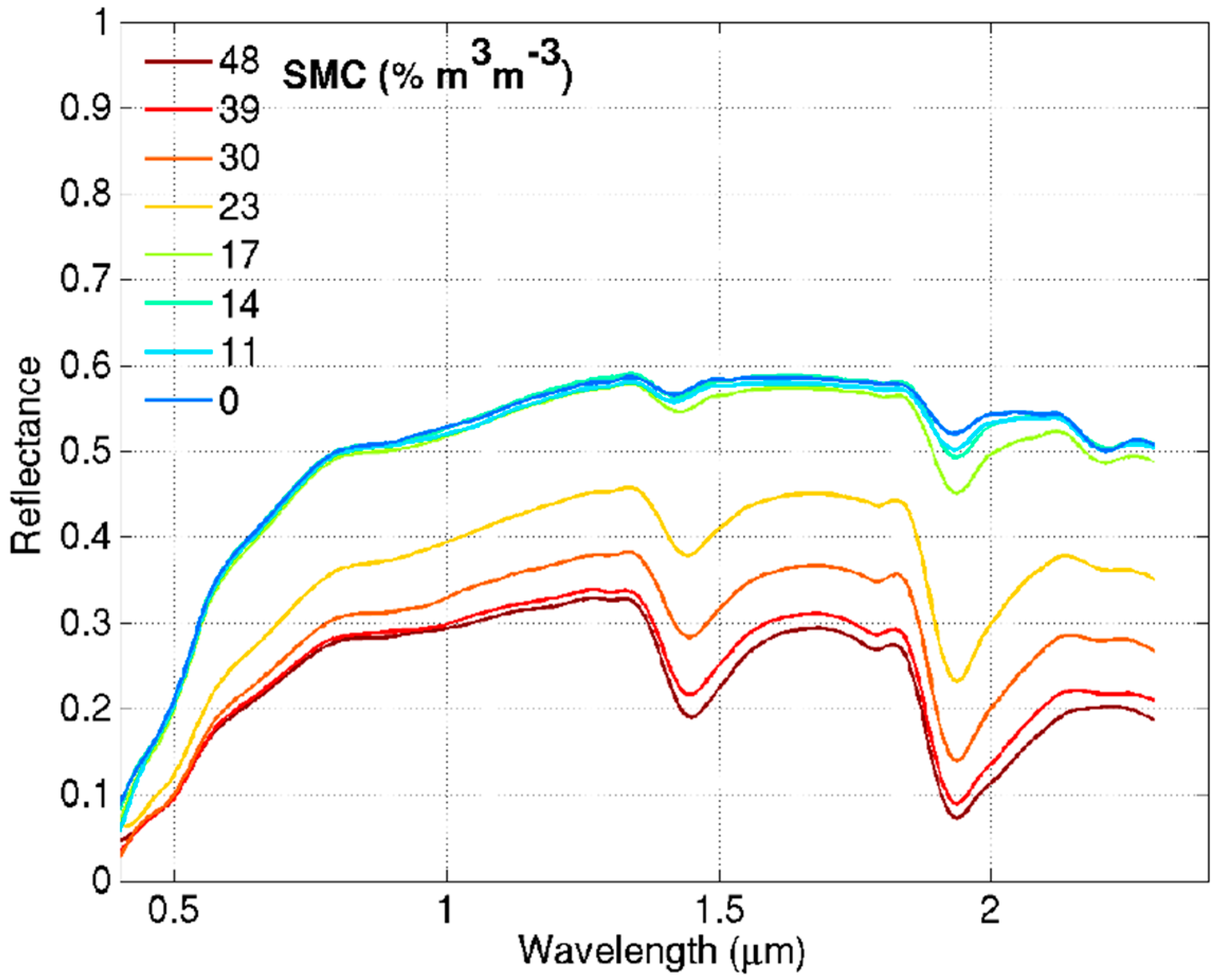
2.4.1. Laboratory Spectra

2.4.2. In-situ Spectra

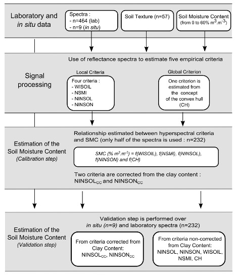
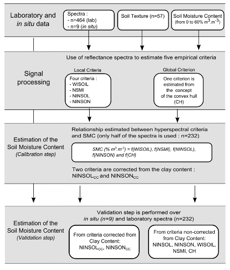
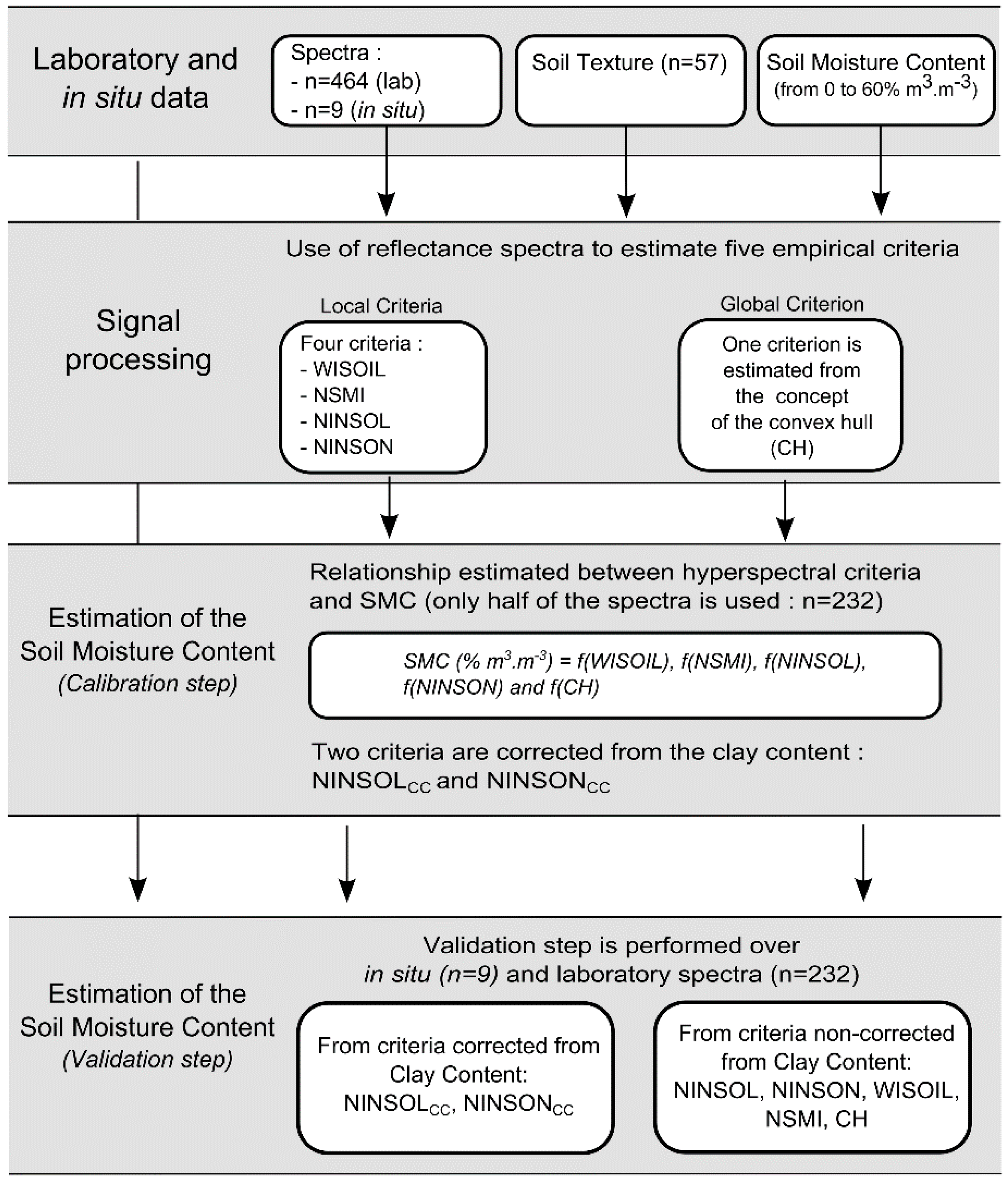
3. Methodology

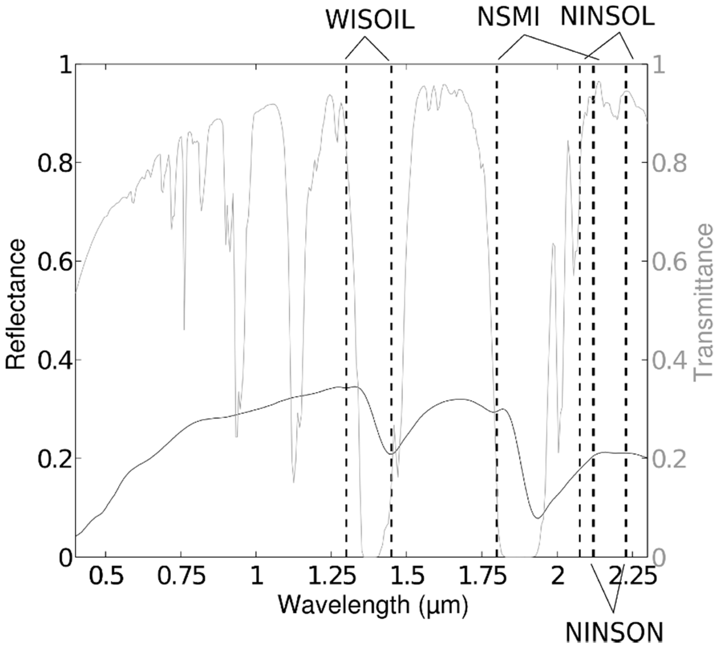
3.1. Local Criteria to Retrieve SMC from Reflectance Spectrum
| Index | λi (µm) | λj (µm) | Type of Regression Function | R2 |
|---|---|---|---|---|
| NSMI | 1.80 | 2.12 | Linear | 0.61 |
| NINSOL | 2.08 | 2.23 | Linear | 0.87 |
| NINSON | 2.12 | 2.23 | Non-linear | 0.87 |

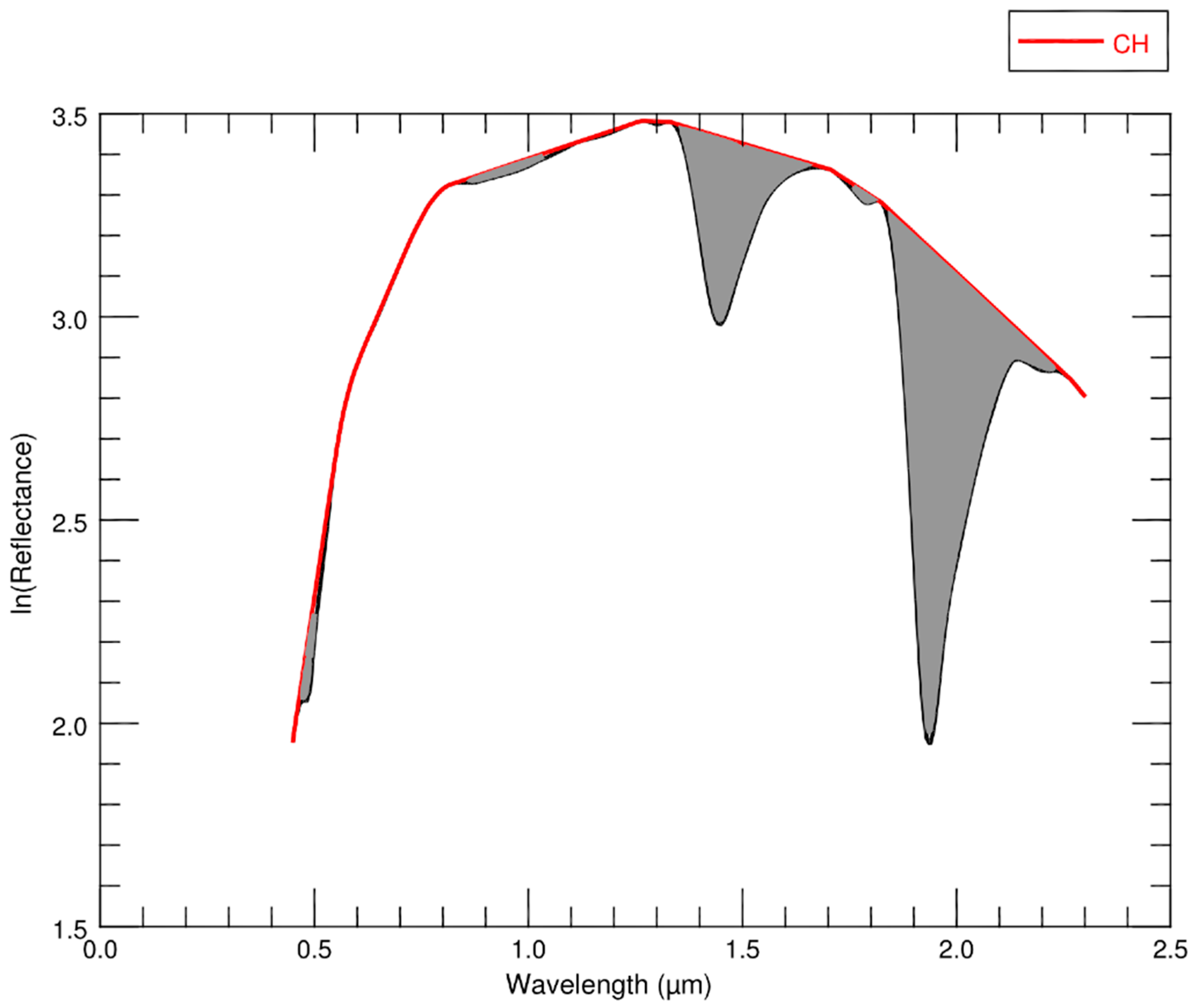
3.2. Global Criteria to Retrieve SMC from Reflectance Spectrum
- (1)
- Generating hull points along the spectrum, excluding the absorption regions of water, clay, other minerals and organic matter,
- (2)
- Calculating the area between the spectrum curve (its natural logarithm) and the CH (see Figure 7 for an example of the CH). This area increases with the SMC because of the presence of the water absorption bands. In these regions the value of the reflectance decreases when the SMC increases and as a consequence, the area between the spectrum and the CH increases,
- (3)
- Estimating the SMC from the area previously calculated, by linking them with a linear regression.

4. Results and Discussions
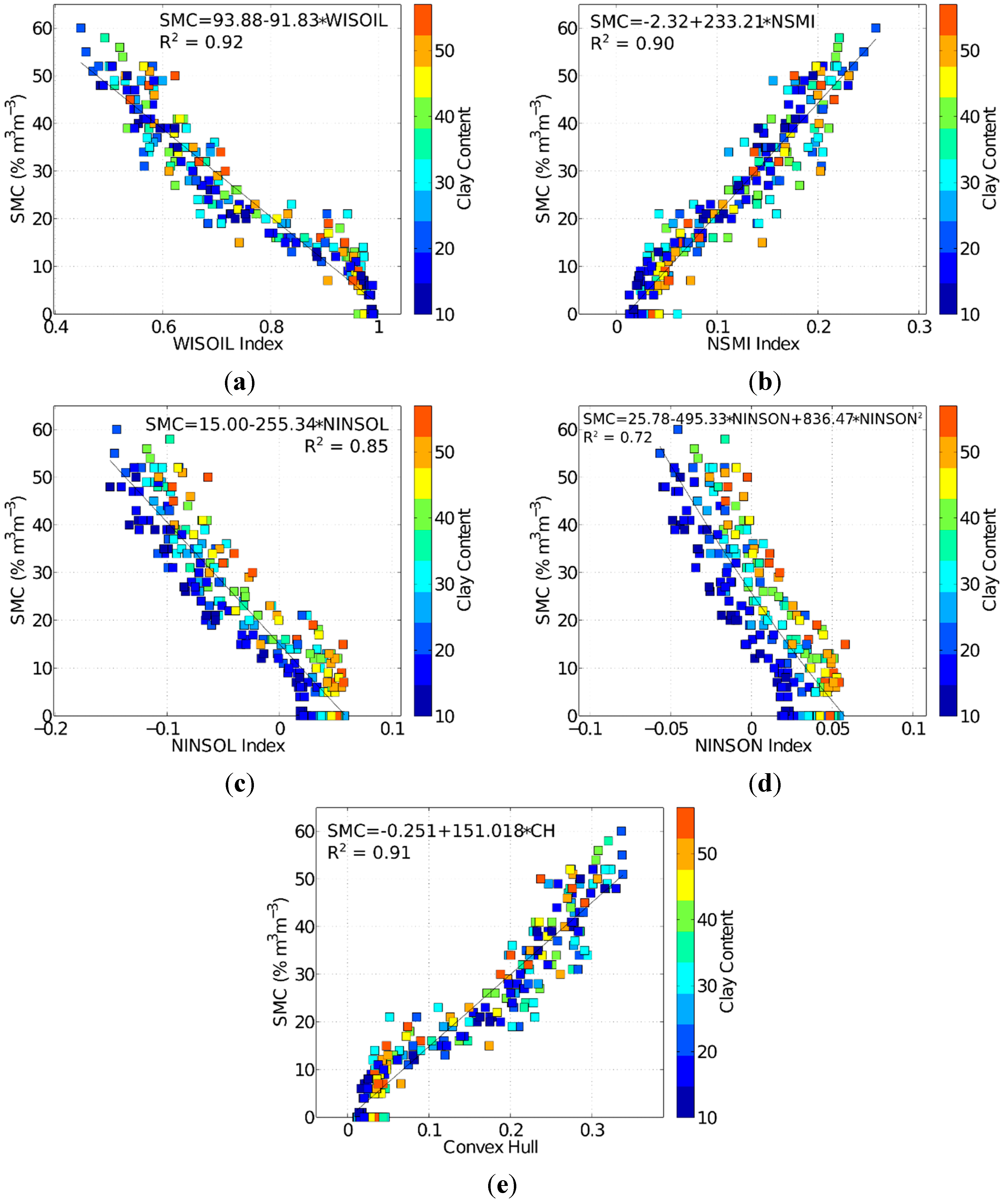
4.1. SMC Retrieval: Calibration Step


4.2. SMC Retrieval: Validation Step
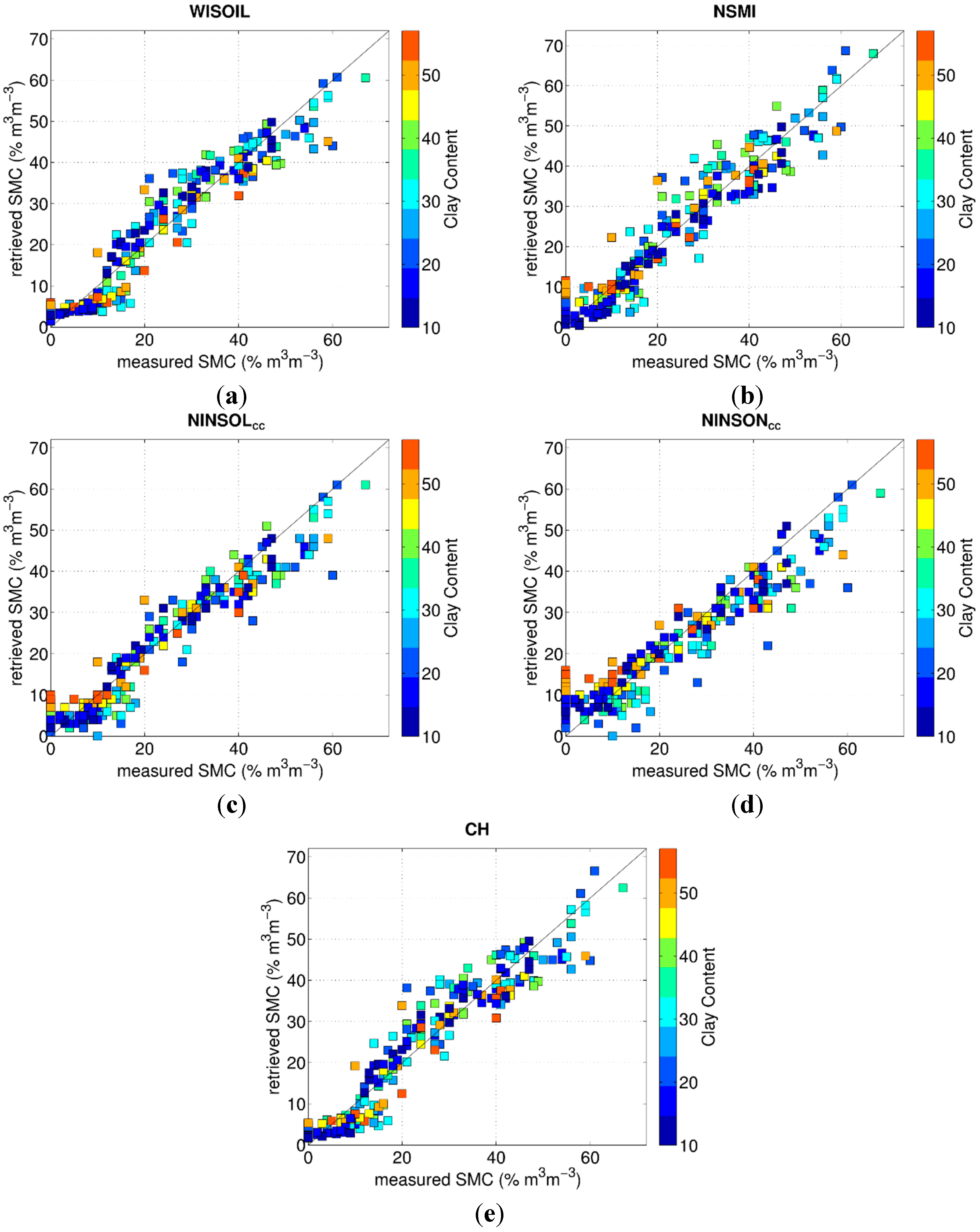
4.2.1. From Laboratory Spectra

| Criteria | Bias (% m3∙m−3) | Stddev (% m3∙m−3) | RMSE (% m3∙m−3) | R2 |
|---|---|---|---|---|
| WISOIL | −0.1 | 4.8 | 4.8 | 0.92 |
| NSMI | 0.2 | 5.4 | 5.4 | 0.90 |
| NINSOL | −0.2 | 6.1 | 6.1 | 0.87 |
| NINSOLCC | −0.7 | 4.9 | 5.0 | 0.92 |
| NINSON | −0.3 | 8.3 | 8.3 | 0.76 |
| NINSONCC | −0.6 | 6.4 | 6.4 | 0.88 |
| CH | 0.0 | 5.1 | 5.1 | 0.91 |
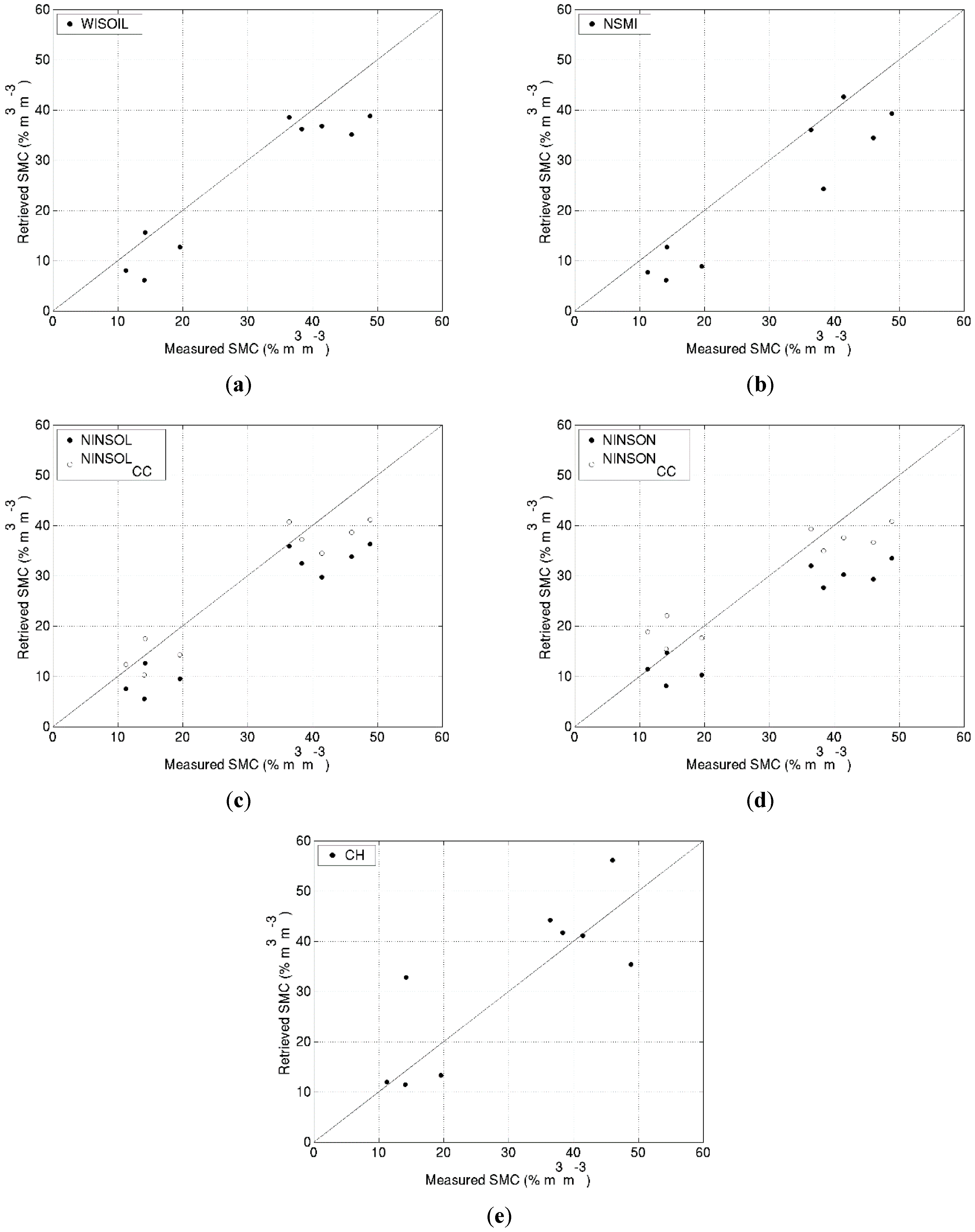
4.2.2. From In-situ Spectra
| Criteria | Bias (% m3∙m−3) | Stddev (% m3∙m−3) | RMSE (% m3∙m−3) | R2 |
|---|---|---|---|---|
| WISOIL | −4.7 | 4.7 | 6.6 | 0.90 |
| NSMI | −6.4 | 5.5 | 8.5 | 0.87 |
| NINSOL | −7.4 | 4.7 | 8.8 | 0.91 |
| NINSOLCC | −2.6 | 4.7 | 5.4 | 0.91 |
| NINSON | −8.1 | 6.2 | 10.2 | 0.89 |
| NINSONCC | −0.8 | 6.2 | 6.2 | 0.89 |
| CH | 2.0 | 9.5 | 9.7 | 0.67 |

5. Conclusions and Perspectives
Acknowledgments
Author Contributions
Conflicts of Interest
References
- Chen, X.; Zhang, Z.C.; Chen, X.H.; Shi, P. The impact of land use and land cover changes on soil moisture and hydraulic conductivity along the karst hill slopes of southwest China. Environ. Earth Sci. 2009, 59, 811–820. [Google Scholar] [CrossRef]
- Munroa, R.K.; Lyonsa, W.F.; Shao, Y.; Wood, M.S.; Hood, L.M.; Leslie, L.M. Modeling land surface atmosphere interactions over the Australian continent with an emphasis on the role of soil moisture. Environ. Model. Softw. 1998, 13, 333–339. [Google Scholar] [CrossRef]
- Chen, L.; Wang, J.; Wei, W.; Fu, B.; Wu, D. Effects of landscape restoration on soil water storage and water use in the Loess Plateau Region, China. For. Ecol. Manag. 2010, 259, 1291–1298. [Google Scholar] [CrossRef]
- Ahmad, S.; Kalra, A.; Stephen, H. Estimating soil moisture using remote sensing data: A machine learning approach. Adv. Water Resour. 2010, 33, 69–80. [Google Scholar] [CrossRef]
- Watson, R.; Moss, R.; Zinyower, M. The Regional Impacts of Climate Change: An Assessment of Vulnerability; IPCC Special Report; Cambridge University: Cambridge, UK, 1998. [Google Scholar]
- Shao, Y.; Henderson-Sellers, A. Modeling soil moisture: A project for intercomparison of land surface parameterization schemes phase 2(b). J. Geophys. Res. 1996, 101, 7227–7250. [Google Scholar] [CrossRef]
- De Roo, A.P.J.; Offermans, R.J.E.; Cremers, N.H.D.T. LISEM a single-event physically based hydrological and soil erosion model for drainage basins II: Sensitivity analysis, validation and application. Hydrol. Process. 1998, 10, 1119–1126. [Google Scholar] [CrossRef]
- Merritt, W.; Letcher, R.; Jakeman, A. A review of erosion and sediment transport models. Environ. Model. Softw. 2003, 18, 761–799. [Google Scholar] [CrossRef]
- Hively, W.D.; McCarty, G.W.; Reeves, J.B.; Lang, M.W.; Oesterling, R.A.; Delwiche, S.R. Use of airborne hyperspectral imagery to map soil properties in tilled agricultural fields. Appl. Environ. Soil Sci. 2011, 2011. [Google Scholar] [CrossRef]
- Ben-Dor, E.; Chabrillat, S.; Demattê, J.A.M.; Taylor, G.R.; Hill, J.; Whiting, M.L.; Sommer, S. Using imaging spectroscopy to study soil properties. Remote Sens. Environ. 2009, 113, 538–555. [Google Scholar] [CrossRef]
- Nocita, M.; Stevens, A.; Noon, C.; Wesemae, B.V. Prediction of soil organic carbon for different levels of soil moisture using Vis-NIR spectroscopy. Geoderma 2013, 199, 37–42. [Google Scholar] [CrossRef]
- Fu, B.J.; Wang, J.; Chen, L.D.; Qiu, Y. The effects of land use on soil moisture variation in the Danangou catchment of the Loess Plateau, China. Catena 2003, 54, 197–213. [Google Scholar] [CrossRef]
- Knapp, A.K.; Fay, P.; Blair, J.; Collins, S.; Smith, M.; Carlisle, J.; Harper, C.; Danner, B.; Lett, M.; McCarron, J. Rainfall variability, carbon cycling, and plant species diversity in a mesic grassland. Science 2002, 298, 2202–2205. [Google Scholar] [CrossRef] [PubMed]
- Kanamitsu, M.; Lu, C.H.; Schemm, J.; Ebisuzaki, W. The predictability of soil moisture and near-surface temperature in hindcasts of the NCEP seasonal forecast model. J. Clim. 2003, 16, 510–521. [Google Scholar] [CrossRef]
- Zhang, W.J.; Lu, Q.F.; Gao, Z.Q.; Peng, J. Response of remotely sensed normalized difference water deviation index to the 2006 drought of eastern Sichuan Basin. Sci. China Ser. D Earth Sci. 2008, 51, 748–758. [Google Scholar] [CrossRef]
- Muller, E.; Decamps, H. Modeling soil moisture reflectance. Remote Sens. Environ. 2000, 76, 173–180. [Google Scholar] [CrossRef]
- Prasad, A.K.; Chaib, L.; Singh, R.P.; Kafatos, M. Crop yield estimation model for Iowa using remote sensing and surface parameters. Int. J. Appl. Earth Obs. Geoinf. 2006, 8, 26–33. [Google Scholar] [CrossRef]
- Nanni, M.R.; Dematte, J.A.M. Spectral reflectance methodology in comparison to traditional soil analysis. Soil Sci. Soc. Am. J. 2006, 70, 393–407. [Google Scholar] [CrossRef]
- Hadria, R.; Duchemin, B.; Jarlan, L.; Dedieu, G.; Baup, F.; Khabba, S.; Olioso, A.; Le Toan, T. Potentiality of optical and radar satellite data at high spatio-temporal resolutions for the monitoring of irrigated wheat crops in Morocco. Int. J. Appl. Earth Obs. Geoinf. 2010, 12, S32–S37. [Google Scholar] [CrossRef]
- Yanmin, Y.; Na, W.; Youqi, Ch.; Yingbin, H.; Pengqin, T. Soil moisture monitoring using hyper-spectral remote sensing technology. In Proceedings of the Second IITA International Conference on Geoscience and Remote Sensing (IITA-GRS 2010), Qingdao, China, 28–31 August 2010; pp. 373–376.
- Vauclin, M. L’humidité des sols en hydrologie: Intérêt et limites de la télédétection. Hydrological Applications of Remote Sensing and Remote Data Transmission, Proceedings of the Hamburg Symposium; IAHS publisher: Wallingford, UK; pp. 401–409. Available online: https://www.itia.ntua.gr/hsj/redbooks/145/iahs_145_0499.pdf (accessed on 19 March 2015).
- Nduwamungu, C.; Ziadi, N.; Tremblay, G.F.; Parent, L.E. Near-infrared reflectance spectroscopy prediction of soil properties: Effects of sample cups and preparation. Soil Sci. Soc. Am. J. 2009, 73, 1896–1903. [Google Scholar] [CrossRef]
- Yang, Z.P.; Ouyang, H.; Zhang, X.Z.; Xu, X.G.; Zhou, C.; Yang, W. Spatial variability of soil moisture at typical alpine meadow and steppe sites in the Qinghai-Tibetan Plateau permafrost region. Environ. Earth Sci. 2011, 63, 477–488. [Google Scholar] [CrossRef]
- Bryant, R.; Thoma, D.; Moran, S.; Holifield, C.; Goodrich, D.; Deefer, T.; Paige, G.; Williams, D.; Skirvin, S. Evaluation of hyperspectral, infrared temperature and radar measurements for monitoring surface soil moisture. In Proceedings of the First Interagency Conference on Research in the Watersheds, Benson, AZ, USA, 27–30 October 2003; pp. 528–533.
- Wagner, W.; Bloshl, G.; Pampaloni, P.; Calvet, J.C.; Bizzarri, B.; Wigneron, J.P.; Kerr, Y. Operational readiness of microwave remote sensing of soil moisture for hydrologic applications. Nord. Hydrol. 2007, 38, 1–20. [Google Scholar] [CrossRef]
- Kerr, Y.H.; Waldteufel, P.; Wigneron, J.P.; Martinuzzi, J.M.; Font, J.; Berger, M. Soil moisture retrieval from space: The Soil Moisture and Ocean Salinity (SMOS) mission. IEEE Trans. Geosci. Remote Sens. 2001, 39, 1729–1735. [Google Scholar] [CrossRef]
- Stamenkovic, J.; Tuia, D.; de Morsier, F.; Borgeaud, M.; Thiran, J.P. Estimation of soil moisture from airborne hyperspectral imagery with support vector regression. In Proceedings of the Workshop on Hyperspectral Image and Signal Processing: Evolution in Remote Sensing (WHISPERS), Lausanne, Switzerland, 25–27 June 2014.
- Peng, J.; Shen, H.; He, S.W.; Wu, J.S. Soil moisture retrieving using hyperspectral data with the application of wavelet analysis. Environ. Earth Sci. 2012, 69, 279–288. [Google Scholar] [CrossRef]
- Kaleita, A.L.; Tian, L.F.; Hirschi, M.C. Relationship between soil moisture content and soil surface reflectance. Trans. Am. Soc. Agric. Eng. 2005, 48, 1979–1986. [Google Scholar] [CrossRef]
- Angström, A. The albedo of various surfaces of ground. Geogr. Ann. 1925, 7, 323–327. [Google Scholar]
- Bach, H.; Mauser, W. Modelling and model verification of the spectral reflectance of soils under varying moisture conditions. In Proceedings of the Geoscience and Remote Sensing Symposium (IGARSS), Pasadena, CA, USA, 8–12 August 1994; Volume 4, pp. 2354–2356.
- Liu, W.; Baret, F.; Gu, X.F.; Tong, Q.; Zheng, L.; Zhang, B. Relating soil surface moisture to reflectance. Remote Sens. Environ. 2002, 81, 238–246. [Google Scholar] [CrossRef]
- Lesaignoux, A.; Fabre, S.; Briottet, X. Influence of soil moisture content on spectral reflectance of bare soils in the 0.4–14 m domain. Int. J. Remote Sens. 2013, 34, 2268–2285. [Google Scholar] [CrossRef]
- Whiting, M.L.; Li, L.; Ustin, S.L. Predicting water content using gaussian model on soil spectra. Remote Sens. Environ. 2004, 89, 535–552. [Google Scholar] [CrossRef]
- Fabre, S.; Briottet, X.; Lesaignoux, A. Estimation of soil moisture content from the spectral reflectance of bare soils in the 0.4–2.5 µm domain. Sensors 2015, 15, 3262–3281. [Google Scholar] [CrossRef] [PubMed]
- Lobell, D.B.; Asner, G.P. Moisture effects on soil reflectance. Soil Sci. Am. J. 2002, 66, 722–727. [Google Scholar] [CrossRef]
- Haubrock, S.N.; Chabrillat, S.; Lemmnitz, C.; Kaufmann, H. Surface soil moisture quantification models from reflectance data under field conditions. Int. J. Remote Sens. 2008, 29, 3–29. [Google Scholar] [CrossRef]
- Hummel, J.W.; Sudduth, K.A.; Hollinger, S.E. Soil moisture and organic matter prediction of surface and subsurface soils using an NIR soil sensor. Comput. Electron. Agric. 2001, 32, 149–165. [Google Scholar] [CrossRef]
- Bruand, A.; Tessier, D. Water retention properties of the clay in soils developed on clayey sediments: Significance of parent material and soil history. Eur. J. Soil Sci. 2000, 51, 679–688. [Google Scholar] [CrossRef]
- Stevens, A.; Udelhoven, T.; Denis, A.; Tychon, B.; Lioy, R.; Hoffman, L.; van Wesemael, B. Measuring soil organic carbon in croplands at regional scales using imaging spectroscopy. Geoderma 2010, 158, 32–45. [Google Scholar] [CrossRef]
- Mulder, V.L.; de Brui, S.; Schaepman, M.E.; Mayr, T.R. The use of remote sensing in soil and terrain mapping—A review. Geoderma 2011, 162, 1–19. [Google Scholar] [CrossRef]
- Haubrock, S.; Chabrillat, S.; Kaufmann, H. Application of hyperspectral imaging for the quantification of surface soil moisture in erosion monitoring and modeling. In Proceedings of the 4th EARSel Workshop on Imaging Spectroscopy, Warsaw, Poland, 27–30 April 2005.
- Finn, M.P.; Lewis, M.; Bosch, D.D.; Giraldo, M.; Yamamoto, K.; Sullivan, D.G.; Kincaid, R.; Luna, R.; Allam, G.K.; Kvien, C. Remote sensing of soil moisture using airborne hyperspectral data. GISci. Remote Sens. 2011, 48, 522–540. [Google Scholar] [CrossRef]
- Sobrino, J.A.; Franch, B.; Mattar, C.; Jiménez-Muñoz, J.C.; Corbari, C. A method to estimate soil moisture from Airborne Hyperspectral Scanner (AHS) and ASTER data: Application to SEN2FLEX and SEN3EXP campaigns. Remote Sens. Environ. 2012, 117, 415–428. [Google Scholar] [CrossRef]
- Wang, Q.; Li, P.; Zhi, P.; Chen, X. Calibration and validation of salt-resistant hyperspectral indices for estimating soil moisture in arid land. J. Hydrol. 2011, 408, 276–285. [Google Scholar] [CrossRef]
- Haubrock, S.; Chabrillat, S.; Kuhnert, M.; Hostert, P.; Kaufmann, H. Surface soil moisture quantification and validation based on hyperspectral data and field measurements. J. Appl. Remote Sens. 2008, 2. [Google Scholar] [CrossRef]
- Lopinto, E.; Ananasso, C. The Prisma Hyperspectral Mission. In Proceedings of the 33rd EARSeL Symposium Towards Horizon 2020: Earth Observation and Social Perspectives, Matera, Italy, 3–6 June 2013.
- EnMAP. Available online: http://www.enmap.org/ (accessed on 27 March 2014).
- Michel, S.; Lefevre-Fonollosa, M.-J.; Hosford, S. HYPXIM—A hyperspectral satellite defined for science, security and defence users. In Proceedings of the Hyperspectral Workshop, ESA-Esrin Frascati, Italy, 17–19 March 2010.
- Baup, F.; Fieuzal, R.; Marais-Sicre, C.; Dejoux, J.-F.; Le Dantec, V.; Mordelet, P.; Claverie, M.; Hagolle, O.; Lopes, A.; Keravec, P.; et al. MCM’10: An experiment for satellite multi-sensors crop monitoring. From high to low resolution observations. In Proceedings of the Geoscience and Remote Sensing Symposium (IGARSS), Munich, Germany, 22–27 July 2012; pp. 4849–4852.
- Béziat, P.; Ceschia, E.; Dedieu, G. Carbon balance of a three crop succession over two cropland sites in South West France. Agric. For. Meteorol. 2009, 149, 1628–1645. [Google Scholar] [CrossRef] [Green Version]
- Dejoux, J.-F.; Dedieu, G.; Hagolle, O.; Ducrot, D.; Menaut, J.-C.; Ceschia, E.; Baup, F.; Demarez, V.; Marais-Sicre, C.; Kadiri, M.; et al. Kalideos OSR MiPy: Un observatoire pour la recherche et la démonstration des applications de la télédétection a la gestion des territoires. Rev. Fr. Photogramm. Télédétect. 2012, 197, 17–30. [Google Scholar]
- Marais-Sicre, C.; Baup, F.; Fieuzal, R. Determination of the crop row orientations from Formosat-2 multi-temporal and panchromatic images. ISPRS J. Photogramm. Remote Sens. 2014, 94, 127–142. [Google Scholar] [CrossRef] [Green Version]
- Gaskin, G.J.; Miller, J.D. Measurement of soil water content using a simplified impedance measuring technique. J. Agric. Eng. Resour. 1996, 63, 153–160. [Google Scholar] [CrossRef]
- European Soil Bureau working group. “HYdraulic PRoperties of European Soils” (HYPRES). Texture Classes. HYPRES Website. Available online: http://www.macaulay.ac.uk/hypres/hypressoil.html (accessed on 29 January 2015).
- Dorigo, W.; Bachmann, M.; Heldens, W. AS Toolbox and Processing of Field Spectra, User’s Manual; German Aerospace Center (DLR): Wessling, Germany, December 2006; Version 1.13. [Google Scholar]
- Khanna, S.; Palacios-Orueta, A.; Whiting, M.L.; Ustin, S.L.; Riao, D.; Litago, J. Development of angle indexes for soil moisture estimation, dry matter detection and land-cover discrimination. Remote Sens. Environ. 2007, 109, 154–165. [Google Scholar] [CrossRef]
- Whalley, W.R.; Leeds-Harrison, P.B.; Bowman, G.E. Estimation of soil moisture status using near infrared reflectance. Hydrol. Process. 1991, 5, 321–327. [Google Scholar] [CrossRef]
- Crowley, J.K.; Brickey, D.W.; Rowan, L.C. Airborne imaging spectrometer data of the Ruby Mountains, Montana: Mineral discrimination using relative absorption band-depth images. Remote Sens. Environ. 1989, 29, 121–134. [Google Scholar] [CrossRef]
- Wold, S.; Sjöström, M.; Eriksson, L. PLS-regression: A basic tool of Chemometrics. Chemom. Intell. Lab. Syst. 2001, 58, 109–130. [Google Scholar] [CrossRef]
- Gomez, C.; Lagacherie, P.; Coulouma, G. Regional predictions of eight common soil properties and their spatial structures from hyperspectral VIS-NIR data. Geoderma 2012, 189, 176–185. [Google Scholar] [CrossRef]
© 2015 by the authors; licensee MDPI, Basel, Switzerland. This article is an open access article distributed under the terms and conditions of the Creative Commons Attribution license (http://creativecommons.org/licenses/by/4.0/).
Share and Cite
Oltra-Carrió, R.; Baup, F.; Fabre, S.; Fieuzal, R.; Briottet, X. Improvement of Soil Moisture Retrieval from Hyperspectral VNIR-SWIR Data Using Clay Content Information: From Laboratory to Field Experiments. Remote Sens. 2015, 7, 3184-3205. https://doi.org/10.3390/rs70303184
Oltra-Carrió R, Baup F, Fabre S, Fieuzal R, Briottet X. Improvement of Soil Moisture Retrieval from Hyperspectral VNIR-SWIR Data Using Clay Content Information: From Laboratory to Field Experiments. Remote Sensing. 2015; 7(3):3184-3205. https://doi.org/10.3390/rs70303184
Chicago/Turabian StyleOltra-Carrió, Rosa, Frédéric Baup, Sophie Fabre, Rémy Fieuzal, and Xavier Briottet. 2015. "Improvement of Soil Moisture Retrieval from Hyperspectral VNIR-SWIR Data Using Clay Content Information: From Laboratory to Field Experiments" Remote Sensing 7, no. 3: 3184-3205. https://doi.org/10.3390/rs70303184