Integration of 2D Lateral Groundwater Flow into the Variable Infiltration Capacity (VIC) Model and Effects on Simulated Fluxes for Different Grid Resolutions and Aquifer Diffusivities

Abstract

Better representations of groundwater processes need to be incorporated into large-scale hydrological models to improve simulations of regional- to global-scale hydrology and climate, as well as understanding of feedbacks between the human and natural systems. We incorporated a 2D groundwater flow model into the variable infiltration capacity (VIC) hydrological model code to address its lack of a lateral groundwater flow component. The water table was coupled with the variably saturated VIC soil column allowing bi-directional exchange of water between the aquifer and the soil. We then investigated how variations in aquifer properties and grid resolution affect modelled evapotranspiration (ET), runoff and groundwater recharge. We simulated nine idealised, homogenous aquifers with different combinations of transmissivity, storage coefficient, and three grid resolutions. The magnitude of cell ET, runoff, and recharge significantly depends on water table depth. In turn, the distribution of water table depths varied significantly as grid resolution increased from 1° to 0.05° for the medium and high transmissivity systems, resulting in changes of model-average fluxes of up to 12.3% of mean rainfall. For the low transmissivity aquifer, increasing the grid resolution has a minimal effect as lateral groundwater flow is low, and the VIC grid cells behave as vertical columns. The inclusion of the 2D groundwater model in VIC will enable the future representation of irrigation from groundwater pumping, and the feedbacks between groundwater use and the hydrological cycle.

1. Introduction

Human water requirement is increasing at the global scale [1] and has significantly modified hydrological processes through irrigation, artificial dams and water diversions [2]. Currently, a third of freshwater withdrawal is derived from groundwater pumping, which provides an estimated 42% of water used for agriculture [3]. Human–water interactions can significantly change the terrestrial water cycle; for example, groundwater-fed irrigation can transform regions from areas of moisture limited to energy limited evapotranspiration (ET), influencing both water and energy budgets [1,2,3,4,5,6].

Examples of extensively irrigated areas are found in the Hau He, Huan He and Yangtse basins in China, along the River Nile in Egypt and Sudan, in the Mississippi–Missouri river basin in USA, and in northern India and Pakistan along the Ganges and Indus rivers [7]. Despite the critical importance of groundwater to global water security [8], the impact of human intervention on the water cycle by groundwater abstraction and groundwater-fed irrigation is not yet fully understood [9]. Feedbacks between the human and natural systems can be complex, such as in the Indo-Gangetic basin where a spatially complex pattern of both groundwater depletion and areas of water logging is observed. This has occurred because of groundwater pumping and complex and dynamic recharge processes influenced by groundwater use, river flows and canal engineering [10]. To improve understanding of feedbacks between the human and natural systems, better representations of groundwater processes need to be incorporated into global/meso-scale hydrological models (GHMs), land surface models (LSMs), and Earth system models (ESMs) [1]. The effects of groundwater abstraction and groundwater-fed irrigation on hydro-climatology has received limited attention, partly because groundwater is either ignored, or represented crudely in such models [8]. Representations of groundwater storage dynamics have been included in a number of model codes. Some calculate changes in groundwater storage based on a mass balance of fluxes and withdrawals [11], some represent groundwater using linear or non-linear reservoirs [2,8,12,13,14], which may or may not simulate the influence of a moving capillary fringe on recharge, and some couple one-dimensional numerical models of unsaturated-saturated flow to the base of the soil column [15,16,17]. However, relatively few models have included lateral groundwater flow, even though it has been recognised as a key missing process [6,8], acting across multiple spatial scales: in humid areas at the hill-slope scale to the basin scale, to larger scales in semi-arid or arid regions where discharge areas can be remote from recharge areas [3].

It has been shown that it is important to include lateral groundwater flow in GHM/LSM to represent components of the hydrological cycle accurately. For example, Chang et al. [18] showed that differences between the observed ratio of transpiration to ET and that simulated by most LSM were predominantly caused by not representing lateral water flow and water vapour diffusion in the soil. Within the Indian context, Chawla and Mujumdar [19] suggested that lower than observed simulated flows in the River Ganges towards the end of the annual recession after the monsoon season were due to the lack of a baseflow contribution from groundwater, which is not represented by the variable infiltration capacity (VIC) macro-scale hydrological model [20,21] they used. This is an important issue as VIC is widely applied at the all-India scale for a range of purposes, for example for reconstructing historical droughts [22], hydrological forecasting [23], and estimation of land-surface fluxes [24].

Despite the importance of groundwater-related processes in large-scale hydrology, groundwater flow, which connects model cells laterally and redistributes water within space, has only recently become a component in some LSM and GHM codes. These include LEAF2-Hydro [25,26], Parflow-CLM [4,15], the linkage of the Community Land Model (CLM) to a two-dimensional saturated groundwater model [27], or PCR-GLOBWB 1&2 [28,29,30].

Whilst the standard version of VIC [20,21] does not simulate groundwater flow, a small number of studies have partially addressed this limitation. Rosenberg et al. [13] enhanced VIC by coupling the simple groundwater model, SIMGM [12], to the base of the soil column. This additional unconfined aquifer store facilitates the simulation of groundwater table dynamics, and baseflow loss as an empirical function of water table depth (WTD) rather than soil moisture, but there remains no lateral connectivity between the grid cells. More recently, VIC was linked to a two-dimensional MODFLOW [31] groundwater model [32], which was subsequently used for catchment drought assessment [33]. This study used a loose coupling approach [34] to link the two models. At each time-step, groundwater discharge through MODFLOW drains is added to the bottom VIC layer, which may cause the two layers above to wet up. The elevations of the drains were set to the land surface height minus the VIC soil thickness, though spatial aggregation of drain flows was required as the two models had different grid resolutions: there were 25 MODFLOW grid cells within each VIC cell. VIC then solves the soil water budget and passes recharge to MODFLOW for the next time-step. Recharge is considered to be equivalent to VIC’s baseflow, which is a non-linear function of the moisture content of the bottom soil layer [35]. By using this iterative approach, a significant improvement in simulated streamflow was obtained. However, calculating groundwater recharge in this way using the VIC baseflow formulation maintains the need to specify three calibration parameters; this is not the case if the saturated aquifer and variably saturated soil are explicitly coupled as in Niu et al. [12]. In summary, groundwater has been represented in VIC by either adding laterally unconnected buckets to the bottom of soil column cells, and calculating groundwater recharge as a function of the water table depth [13], or by loosely coupling a 2D groundwater model to VIC without implementing a dynamic recharge formulation [32].

In this study, we extended the previous approaches by integrating a 2D groundwater model into the VIC code, implementing soil moisture–groundwater table interaction according to Niu et al. [12], and enabling direct river–aquifer interaction. This allows the simulation of baseflow contributions to rivers from diffusive groundwater flow through an aquifer and will facilitate the inclusion of more realistic groundwater irrigation schemes based on knowledge of actual practice [36,37], especially within India [38,39,40], representing feedbacks between groundwater pumping, groundwater levels and irrigation return flows. Baseflow to rivers can be modelled either using a groundwater level-dependent Darcian flux, or be allowed to discharge at the land surface when the soil completely saturates. Using this enhanced version of VIC, we then considered how the spatial resolution of the mesh affects lateral groundwater flow, and how it modifies runoff, baseflow, ET, recharge, and WTD. Furthermore, we also investigated how these fluxes and the groundwater table vary when the diffusivity of the aquifer is altered in addition the model grid size, which has not been investigated previously in a two-way integrated model of land surface and groundwater, representing both groundwater recharge and capillary rise. These simulations are based on an idealised representation of the upper Ganges catchment within India.

2. Materials and Methods

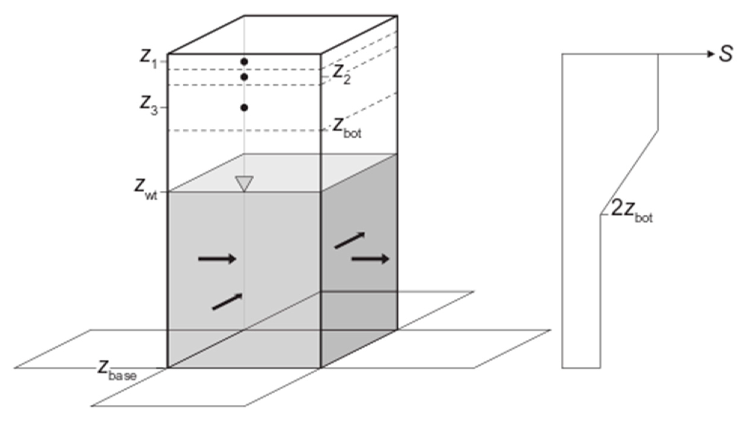
2.1. Implementation of Groundwater Flow Model in VIC

VIC is a macro-scale hydrological model and has been widely applied from basin to global scale for water and energy balance studies in the US, the Arctic and globally (see [20] for a review). The model describes vertical water transport in areally large and thin cells. Sub-grid heterogeneity of land cover and elevation is handled with statistical distributions of the different land cover types and elevation bands, dividing a cell into a number of tiles. For each of these tiles, ET, infiltration, runoff, soil moisture and baseflow are calculated separately and weighted by area to give a cell-average value for each variable. The water and energy balance for each grid cell is solved independently and there is no lateral connectivity between the cells. The runoff function within VIC calculates surface runoff, infiltration, soil water transport and baseflow as follows: when precipitation reaches the land surface, it is partitioned into runoff and infiltration, according to the variable infiltration curve [41]. It assumes that surface runoff from the upper two soil layers is generated by those areas for which precipitation and the soil moisture exceeds the storage capacity of the soil. Water is calculated to flow between the soil layers using a 1D Richards equation [42], assuming free drainage and using the Brooks–Corey relationship for hydraulic conductivity [42]. Baseflow, which leaves the soil column, is calculated as a function of relative moisture of the bottom soil layer according to the Arno model formulation [35]. Routing of runoff and baseflow is performed a posteriori by post-processing model output [43].

Here, we incorporate a two-dimensional model of groundwater flow into the VIC code. This has been based on the AMBHAS code [44]. We do this within the image version of VIC 5.0.1. [20,21], an additional later version of the code, which iterates across each cell before progressing the solution to the next time-step. This “space before time” implementation is required to be able to integrate a distributed groundwater model. In contrast, the classic version of VIC has a “time before space” implementation, solving all time steps for one model cell before moving onto the next cell, which makes linking with a distributed model impossible without changing the entire model structure. In summary, we turn off the VIC algorithm, which calculates baseflow as a function of the soil moisture of the lowest soil layer, and instead calculate the downward recharge, or upward discharge, of water across the base of the VIC soil column at each time-step. This vertical flux is a function of the VIC soil moisture content and the current level of the water table simulated by the groundwater model. This vertical flux is then applied to the groundwater model, which solves for groundwater flow, baseflow to rivers, and the elevation of the water table across the domain for the time-step. Henceforth, we use the term discharge to mean an upward flux of water across the base of the soil column, i.e., a negative recharge. We run the model on a Linux HPC and make use of the VIC parallelisation using MPI. The groundwater model runs on a single processing core, and data are passed between VIC and the groundwater model at each time-step.

2.1.1. Groundwater Model Formulation

We implemented an explicit, or forward-difference [45] two-dimensional, one-layer groundwater model, which solves the following governing partial differential equation of flow:

$$\frac{\partial }{\partial x}\left(T\frac{\partial h}{\partial x}\right)+\frac{\partial }{\partial y}\left(T\frac{\partial h}{\partial y}\right)=S\frac{\partial h}{\partial t}-q_r+q_p+q_b$$

(1)

where $h$ is hydraulic head [L], $T$ is aquifer transmissivity [L²/T], $S$ is the dimensionless aquifer storage coefficient, $q_r$ is groundwater recharge [L/T], $q_p$ is groundwater pumping [L/T], and $q_b$ is baseflow to rivers [L/T]. The aquifer is isotropic but can be heterogeneous. $T$ can be constant in time, or recalculated at the end of each time-step as the saturated aquifer thickness varies, according to:

$$T=K \left(h-z_{base}\right)$$

(2)

where $K$ is hydraulic conductivity [L/T], and $z_{base}$ [L] the elevation of the base of the aquifer, which can both vary spatially. If $T$ is specified to be constant in time, and $S$ set to a confined storage coefficient value, the model can be considered to represent confined aquifers. However, as described subsequently, in the current implementation of the code all groundwater model grid cells are coupled to the VIC soil column using the simulated groundwater level.

The solution of the set of finite difference approximations to Equation (1) on the model grid makes use of a simple operator splitting method [46], which involves three steps: the hydraulic head is updated for recharge and abstraction; then, for baseflow to rivers; finally, for lateral groundwater flow between cells. The time-step length, $\Delta t$, of the groundwater model is adaptive, and adjusted according to the stability criterion $\Delta t\le 0.25\Delta x^{2}S/T$ [47], where $\Delta x$ is the smallest mesh spacing in the grid. To enhance stability of the model solution when the groundwater table is near to the base of the VIC soil, the storage coefficient is set to vary linearly from that of the soil to that of the aquifer, between the base of the soil and twice its depth (Figure 1). Currently, only constant head (Dirichlet-type) and no flow (Neumann-type) boundary conditions can be specified at the lateral edges of the groundwater model domain.

2.1.2. Vertical Soil Water–Groundwater Interaction

Vertical water fluxes between the saturated aquifer and the soil are simulated using the scheme of Niu et al. [12], who incorporated a simple groundwater model, SIMGM, into version 2.0 of CLM [48].

If the water table is below the base soil column, recharge, $q_r$ [L/T], is calculated as:

$$q_r=-K_a\frac{-z_{wt}-\left({\psi }_{bot}-z_{bot}\right)}{z_{wt}-z_{bot}}$$

(3)

where $K_a$ is the aquifer saturated hydraulic conductivity [L/T], $z_{wt}$ is the water table [L] depth calculated by the groundwater model, $z_{bot}$ is the depth [L] to the base of the soil column, and ${\psi }_{ bot}$ is the matric potential [L] of the bottom soil layer, calculated from the soil moisture characteristic or moisture release curve after Campbell [49]:

$$\psi ={\psi }_e{(\frac{\theta }{{\theta }_s})}^{-b}$$

(4)

where ${\psi }_e$ is the air entry water potential [L], $\theta$ is the volumetric water content [-], ${\theta }_s$ is the saturated water content [-], and $b$ is the slope of ln $\psi$ versus $\ln \theta$. $q_r$ is positive when water infiltrates to the aquifer, but Equation (3) models both downward recharge and the upward flux of water driven by capillary forces. The above recharge formulation is only valid, if the water table is below the soil column. If the water table is within the soil column, recharge, $q_r$, is calculated from the soil layer above that containing the water table as:

$$q_r=-K_{i,wt}\frac{({\psi }_{sat}-z_{wt})-\left({\psi }_i-z_i\right)}{z_{wt}-z_i}$$

(5)

where $K_{i,wt}$ is the hydraulic conductivity between layer $i$ and the water table, ${\psi }_{sat}$ is the capillary head, ${\psi }_i$ is the matric potential of the layer above the water table, $z_i$ is the node depth of the layer above the water table [12] $K_{i,wt}{\psi }_{sat}{\psi }_i{z}_i$.

During testing of the implementation of this algorithm within VIC, we made two modifications to address some occasional erroneous behaviour related to the inherent time-stepping nature of the model. First, water entering the soil column from the aquifer was specified to always contribute to the bottom soil layer, rather than the layer the water table is interacting with. If the bottom soil layer is fully saturated, the runoff function within VIC will redistribute this water upwards. After the runoff function has calculated surface runoff, infiltration, soil water transport and groundwater recharge, the saturation for each soil layer is compared against the residual and maximum saturation, and moisture is moved to the layer above if the saturation is above one. This adjustment ensures that the water table cannot be close to the soil surface whilst the bottom soil layer is not fully saturated. Second, it was found for some model parameterisations that if the water table rose to just below the base of the soil column, large downward vertical gradients were generated causing the lowest soil layer to totally drain. To mitigate this, we introduced a parameter that limits the flux out of the bottom soil layer to a fraction of its moisture content. Appropriate values of this factor will depend on the time-step length and vertical discretisation of the soil column, but 1% was found to be effective for the 2 m deep soil and 3-h time-step used in this study.

2.1.3. River–Groundwater Interaction

Groundwater discharge to the land surface can occur when the groundwater table fully saturates the soil. In this case, the upward groundwater flux will be added to runoff. This may occur anywhere across the model domain. However, we also incorporated a groundwater head-dependent leakage boundary condition (Cauchy type) to represent groundwater interaction with rivers, which can be applied in specific grid cells. This flux, $q_b$ [L/T] in Equation (6), is calculated as:

$$q_b=\{\begin{array}{ll}{c}_i\left(h-h_r\right) ,& for h\ge h_r\\ c_e\left(h-h_r\right) ,& for h_r>h>\left(z_b-B\right)\\ c_e\left[\left(z_b-B\right)-h_r\right] ,& for h\le \left(z_b-B\right)\end{array}$$

(6)

where: $h$ is the groundwater head [L]; $h_r$ is the river stage [L]; $z_b$ and $B$ are the elevation and thickness of the riverbed [L], respectively; $c_i$ and $c_e$ are the conductance [/T] of the riverbed when it gains water from the aquifer (influent), or recharging the aquifer (effluent), respectively. Conceptually, this conductance is considered to be the hydraulic conductivity of the riverbed, which is conceptualised to differ between influent and effluent conditions, divided by its thickness. To calculate the volumetric flow rate, $q_b$ is multiplied by two parameters specifying the width of the rivers within the cell, and their total length. Similar representations of river–aquifer interactions are included in widely-applied groundwater modelling codes (e.g., MODFLOW [31]; FeFlow [50]; ZOOMQ3D [51]). Other LSMs or GHMs coupled with a groundwater model have also used a head-dependent Darcian flux between the river and aquifer [26,29,52], or else, river baseflow has been estimated as the sum of lateral flow reaching one cell [25].

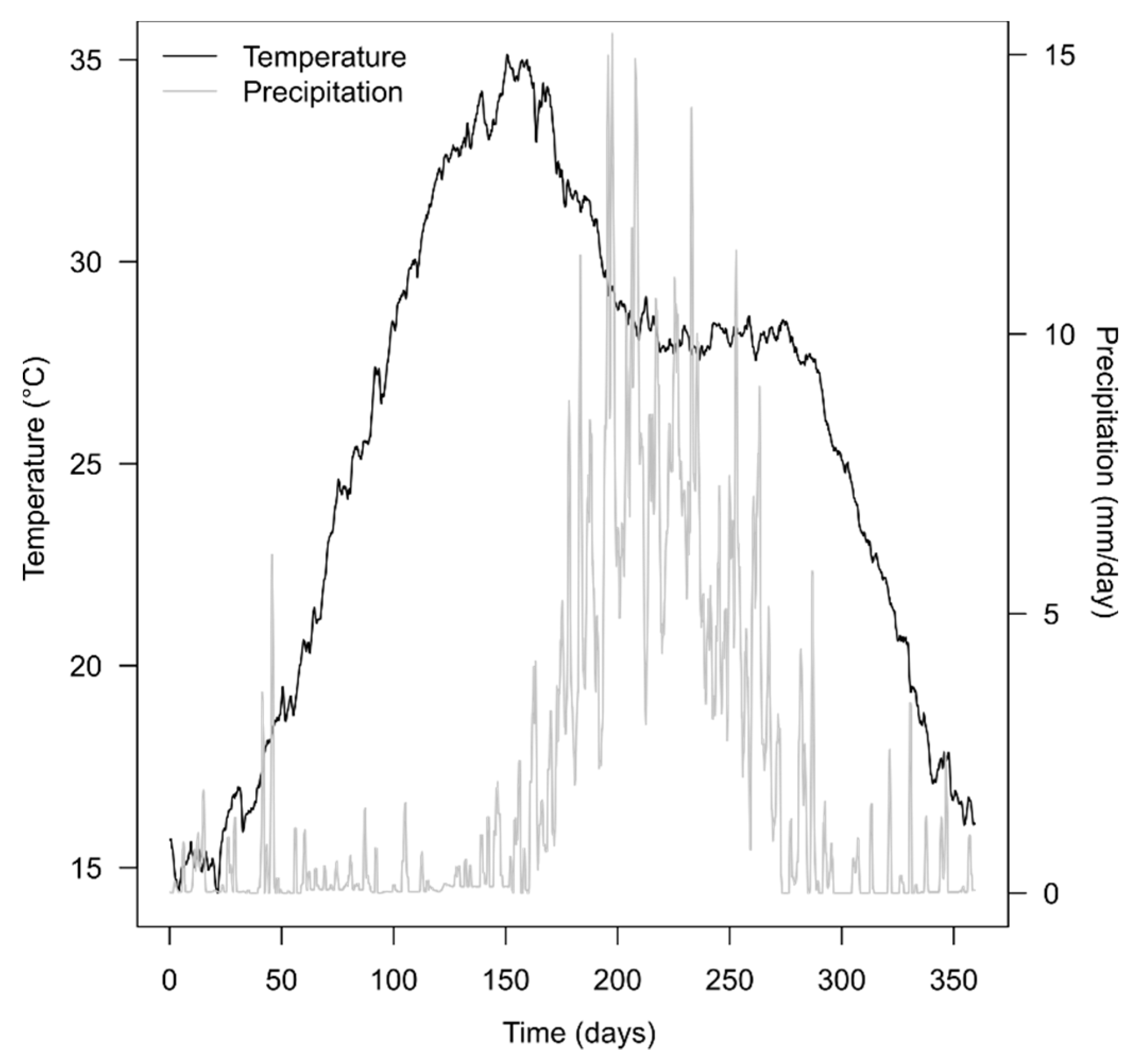
2.2. Model Application

To investigate how the spatial resolution of the mesh affects lateral groundwater flow and how it modifies runoff, baseflow, ET, recharge, and WTD, we apply the model to an idealised system based on the 623,985 km² catchment of the River Ganges within India above the city of Patna (Figure 2). This model is then used to examine how these fluxes and the groundwater table vary when the diffusivity of the aquifer, considered here as the ratio of $T$ and storage coefficient [53], is modified.

The model is homogenous, except for the topographic elevation, and all forcing data are applied uniformly over the model area. This enabled the analysis of the impact of groundwater flow alone, without the complexity arising from heterogeneous parameter and forcing data. The elevation of the land surface, derived from the SRTM digital elevation model [54], varies from 1500 metres above sea level (m asl) in the south-east of the catchment to 50 m asl at Patna (Figure 2). Broadly, the areas of higher ground in the south-west of the catchment correlate with harder igneous rocks, for example, the basalt lavas of the Deccan Traps [55], and the lower-lying areas are associated with the thick alluvial floodplain of the River Ganges.

The model parameters are based on the global VIC parameter dataset [56], and forcing data from the WATCH dataset [57], both extracted at 77.75° E, 25.75° N. The forcing data are air temperature, total precipitation, atmospheric pressure, incoming shortwave radiation, incoming longwave radiation, vapour pressure and wind speed. We calculated averages of the forcing data for each day of the year using the 24 values from the years 1979 to 2002. The resulting annual sequence was then applied repeatedly until a dynamic equilibrium was reached, i.e., when there was no difference in the simulated results for successive years. The mean rainfall is 61.6 mm/month and varies between 10.0 mm/month for the January to March (JFM) period and 192.7 mm/month over July to September (JAS) (Figure 3). Only the modelled data for the last year of the simulation were analysed.

We constructed nine models with the different aquifer diffusivities listed in

Table 1. Model aquifer properties.

Model	Hydraulic Conductivity (m/day)	Storage Coefficient (-)	Maximum Diffusivity (m2/day)
R1	0.1	0.01	5000
R2	0.1	0.1	500
R3	0.1	0.2	250
R4	1	0.01	50,000
R5	1	0.1	5000
R6	1	0.2	2500
R7	10	0.01	500,000
R8	10	0.1	50,000
R9	10	0.2	25,000

, and simulated the catchment at three different grid resolutions: 1°, 0.25°, and 0.05°. In this region of India, these resolutions correspond to grid cell widths of on average 110.8, 24.8, and 5.5 km, and cell heights of on average 99.5, 27.7, and 4.9 km, respectively; there are 58, 924, and 23,151 active grid cells in the three model grids. At each resolution, the surface elevation of each VIC cell was defined to be the mean of the SRTM DEM pixels within the cell. The aquifer was set to be 500 m thick and therefore the maximum $T$ of the models ranges from 50 to 5000 m²/day. The diffusivity of the nine models ranges from 250 to 5 × 10⁵ m²/day. The bases of the three soil layers were set at depths of 0.1, 0.5, and 2 m. Only one elevation band and vegetation type were applied within each grid cell, i.e., there is no sub-grid variability within VIC. No river boundary conditions were defined in any of these simulations, and so where groundwater discharged to the land surface it did so through the soil. However, one further simulation of the R5 model (Table 1) at a resolution of 0.05° was run, in which river boundary conditions were applied in all grid cells. The stage of the river was set to 4 m below the surface in all cells, and a riverbed thickness of 1 m, and conductance of 1 m²/day applied uniformly. Assuming the width of the river to be 100 m, and its length to be the same as the grid cell width, the riverbed hydraulic conductivity would then be approximately 50 m²/day. This is indicative of well-connected river and aquifer.

3. Results

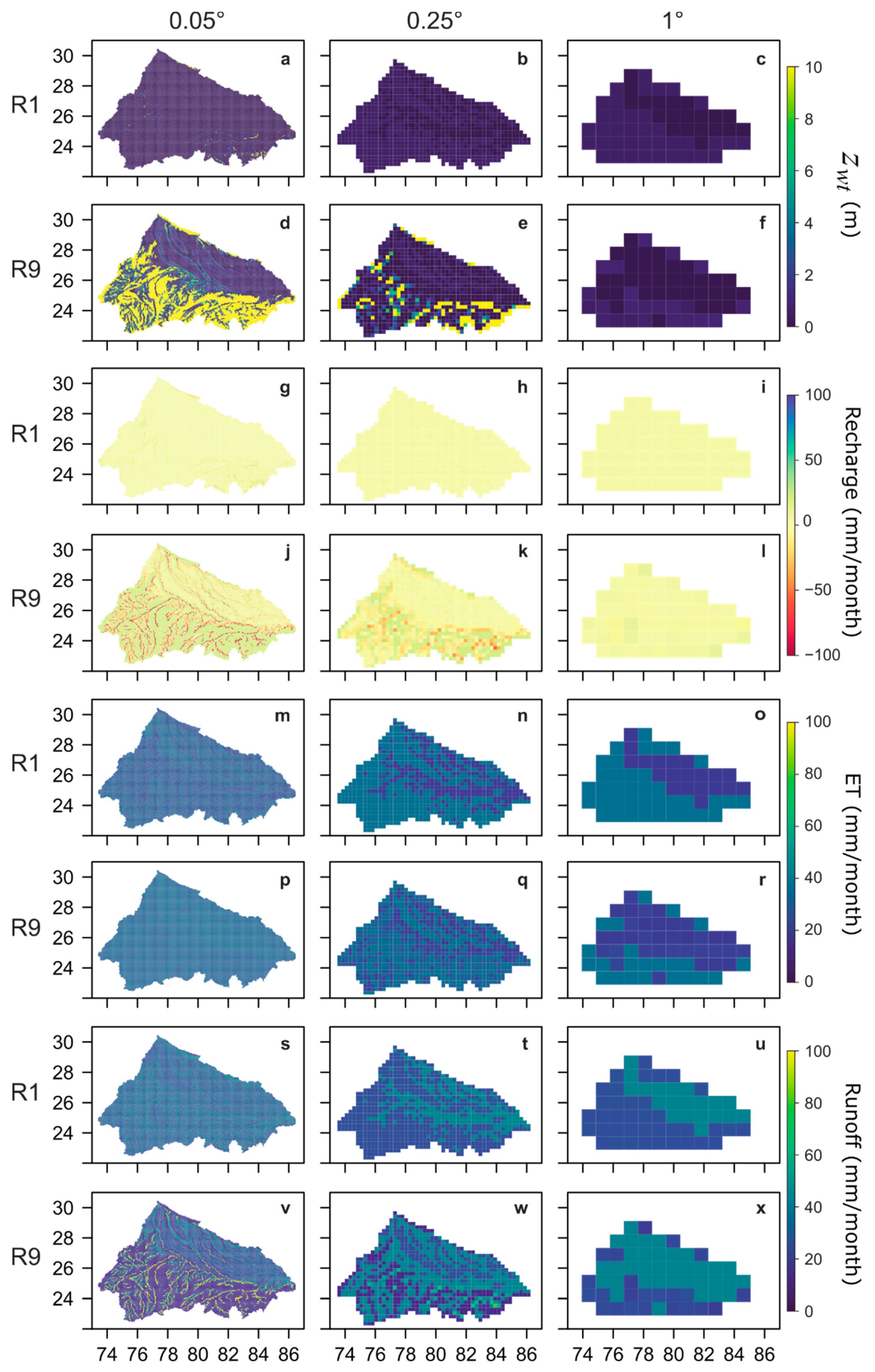
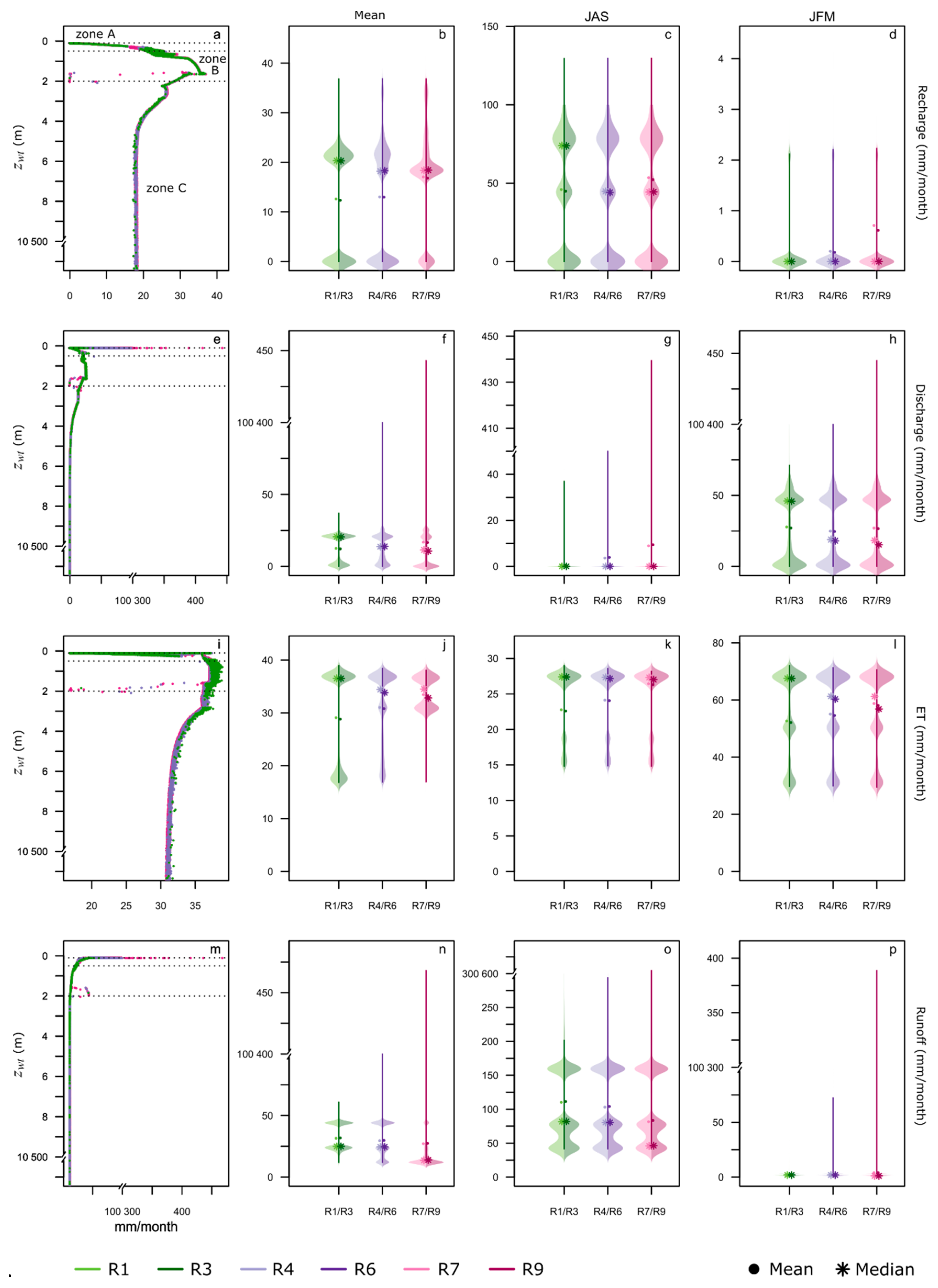
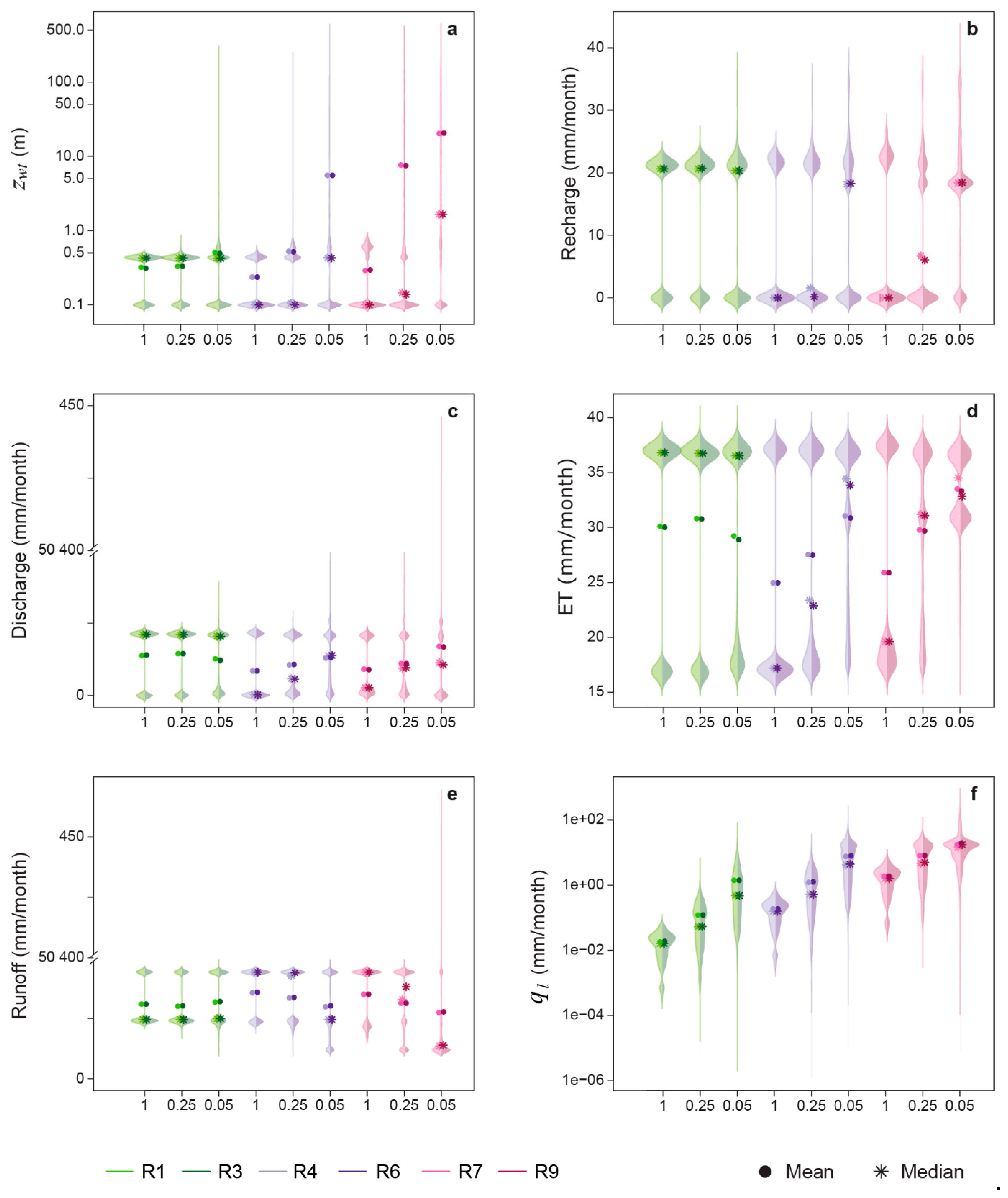
3.1. Effect of Aquifer Properties on Water Table Depth and Fluxes at 0.05 Resolution

Spatial plots of mean water table depth, recharge, ET, and runoff are presented in the first column of Figure 4, for two runs at the 0.05° resolution: R1 with the lowest, and R9 with the highest, values of hydraulic conductivity and storage coefficient. Spatial averages of these mean values are listed in

Table 2. Mean annual water table depth (WTD), model fluxes, and discharge area fraction for Runs 1–9 on the 0.05° grid.

Run	Mean WTD (m)	Mean Recharge (mm/month)	Mean ET (mm/month)	Mean Runoff (mm/month)	Mean Discharge Area Fraction
1	0.52	12.7	29.19	31.89	0.63
2	0.51	12.44	28.94	32.14	0.63
3	0.51	12.42	28.92	32.17	0.63
4	5.65	13.11	31.11	29.97	0.51
5	5.59	13.05	30.9	30.18	0.51
6	5.59	13.07	30.89	30.19	0.51
7	20.41	17.13	33.55	27.55	0.29
8	20.34	16.93	33.35	27.75	0.29
9	20.34	16.89	33.27	27.82	0.29

for all nine model runs.

3.1.1. Water Table Depth

For R1, in which $T$ ≤ 50 m²/day, the simulated mean water table is shallow, and within the VIC soil column across 99% the modelled area. It is in the top-soil layer over 41% of the area, and on average only 0.52 m below ground level (m bgl). The 1st and 99th percentiles of the mean WTD are 0.1 and 2.2 m bgl. Whilst the aquifer storage coefficient is low (1%), because the water table is generally within the soil, which has a porosity of 48.51%, it fluctuates by between only 0.35 and 0.7 m over the year. On average, the water table is deepest in May and shallowest in September after the monsoon season.

In contrast, for R9, in which $T$ ≤ 5000 m²/day, the simulated water table is, as expected, flatter, which results in a larger spatial variation in WTD; the 1st and 99th percentiles are 0.1 and 231 m bgl. The mean WTD is 20.34 m bgl, though across the flatter floodplain of the Ganges it is mostly within 2 m of the land surface. Across 52% of the domain, the mean WTD is within the soil, and across 21% of the catchment it is within the top-soil layer. In R9, the water table again only fluctuates by a limited amount (20.56 to 20.12 m), which in this simulation is partially because of the high storage coefficient (20%) applied when the water table drops below the soil. The water table is deepest in May and shallowest in September after the monsoon season. As would be expected, for the series of three simulations in which the hydraulic conductivity is the same (R1–3, R4–6, and R7–9), the storage coefficient has little effect on the mean WTD.

3.1.2. Groundwater Recharge

The flux across the soil-aquifer boundary consists of drainage by gravity and capillary rise, driven by the interaction between the water table and soil moisture. We refer to a downward flux as recharge, but its sign can be negative, in which case we also use the term discharge to refer to an upward flux. The total mean annual flux across the soil-aquifer boundary is zero for this dynamic equilibrium simulation.

The mean groundwater recharge increases with increasing mean WTD, from 12.7 mm/month for R1 to 16.89 mm/month for R9 (Table 2) (Figure 4g,j). This is, in part, related to shallower water tables causing the soil to become water-logged and transpiration to decrease; in R1, the mean water table is within the top soil layer across 41% of the catchment, whereas this is the case for only 21% of the catchment area in R9. The relationship between the WTD and recharge also affects the difference in mean recharge between the simulations. In Figure 5a, mean WTD is plotted against mean recharge for those models cells where the flux is on average downward. Recharge increases from zero to a maximum value as the WTD increases to approximately 1.5 m, i.e., towards the base of the soil column zone A (Figure 5a). Recharge then decreases as WTD increases to approximately 5 m (zone B). Recharge remains constant for higher WTD as the vertical hydraulic gradient becomes one (zone C). Within the soil, the hydraulic properties are constant with depth, and therefore, the relationship between recharge and WTD is driven by the physical description of Equation (3) and (5). Cell-mean groundwater recharge has a bimodal distribution (Figure 5b), with the two maxima associated with water-logged or discharging cells (zone A), or a downward flux (zones B and C). During the JAS monsoon season, mean recharge is higher, and there is a distinct tri-modal distribution of recharge, with maxima associated with: near-zero values where the water table is shallow (zone A); free drainage-limited recharge rates for deep water tables (zone C), and higher values of approximately 75 mm/month where the water table is close to the soil-aquifer boundary (zone B). During the dry season, there is very little recharge (Figure 5d).

Groundwater discharge through the soil to the land surface is highest when the water table is very shallow, and decreases to zero as the WTD reaches approximately 5 m (Figure 5e). Mean groundwater discharge increases with increasing $T$ as more groundwater flows laterally to fewer discharging cells (Table 2); the mean discharge rate increases by approximately one third, from 12.7 mm/month in R1 to 16.89 mm/month in R9. This is associated with a reduction in the mean discharge area fraction, or proportion of the model domain discharging, from 0.63 to 0.29. Total groundwater discharge is highest during the dry season when the distribution of cell discharge rates is bimodal (Figure 5h): near-zero, or approximately 50 mm/month (~82% of mean rainfall). The lowest discharge rates occur during the wet season, when a greater proportion of the aquifer receives recharge, and a cell is either recharging or discharging at any one time. The extreme values for discharge remain similar between the wet and the dry season (Figure 5g,h), implying that discharge to river valleys is maintained all year round. Similar to the mean annual values, the extreme discharge values for both the wet and dry season increase with increasing aquifer $T$ (Figure 5f–h).

For the low hydraulic conductivity aquifer (R1), the water table is within the soil across the entire model domain, resulting in recharge during the wet season and discharge during the dry season and little lateral flow. This is evident in Figure 4g as the mean annual flux across the soil-aquifer boundary is zero for most of the model domain. In contrast for the high hydraulic conductivity aquifer, lateral groundwater flow results in perennial discharge at certain locations in addition to the seasonal signal of recharge during the wet season and discharge during the dry season.

3.1.3. Evapotranspiration

The mean ET across the catchment increases from 29.19 mm/month (R1) to 33.27 mm/month (R9) as T increases (Table 2). This is because when the soil is waterlogged, transpiration reduces (Figure 4m,p). The relationship between ET and WTD is shown in Figure 5i. ET increases to a maximum as the water table lowers within the soil column. As the WTD increases above approximately 3 m, the contribution of groundwater to ET reduces until it approaches a constant value determined by the soil water balance alone.

The distribution of cell-mean ET (Figure 5j–l) is again tri-modal, because it controlled by the groundwater table-influenced soil moisture content in the three soil zones, A–C. For the low T aquifer (R1–3), the soil is mostly either water-logged (zone A), or the water table is within the soil column (zone B). Consequently, ET values are generally either at the low or high end of the distribution. In contrast for the higher T aquifer (R7–9), the water table is either within zone B of the soil column or deeper. In these runs, ET either occurs at approximately its maximum rate, or at the medium rate related to when the water table is deep and the capillary fringe does not contribute to the soil moisture. Seasonally, the mean ET is lower during the wet season and higher in the dry season in comparison with the mean annual values.

3.1.4. Runoff

Mean annual runoff is higher for R1 (31.89 mm/month) than for R9 (27.82 mm/month) (Table 2). The shallow water table for R1 results in a reduction in transpiration, and hence a higher soil moisture and a higher runoff compared to runs with a deeper water table. Therefore, runoff is high where ET is low and vice-versa. The spatial variation in cell mean runoff is lower with a lower T: the 1st and 99th percentiles are 12.4 and 44.2 mm/month, respectively, for R1, compared 11.9 and 168.2 mm/month for R9. This is because, for a higher hydraulic conductivity aquifer, groundwater flows to topographic low-lying areas, resulting in higher runoff at these locations. Seasonally, mean runoff is high (110.8/84 mm/month for R1/R9) during the wet season, and lower during the dry season (2.3/4.4 mm/month for R1/R9). The extreme values for R9, however, remain high during the dry season.

3.2. Impact of Grid Resolution on Water Table Depth and Water Fluxes

This section presents the impact of grid resolution for different water fluxes and WTD for different aquifer $T$ values. Spatial plots of mean WTD, recharge, ET, and runoff are presented in Figure 4, cumulative distribution functions of WTD at different grid sizes in Figure 6, density distributions of WTD, groundwater recharge, groundwater discharge, ET, runoff and lateral groundwater flow for the different grid resolutions are presented in Figure 7, spatial plots of lateral groundwater flow for the three different grid resolutions in Figure 8, and spatial averages of cell-mean values are listed in

Table 3. Mean WTD, recharge, ET, runoff and lateral groundwater flow for three runs and the three grid resolutions.

Run	Grid Size	Mean WTD (m)	Mean Recharge (mm/month)	Mean ET (mm/month)	Mean Runoff (mm/month)	Mean Lateral Groundwater Flow (mm/month)	Mean Discharge Area Fraction
1	1°	0.32	13.9	30.07	31.03	0.02	0.67
1	0.25°	0.33	14.79	30.86	30.21	0.13	0.65
1	0.05°	0.52	12.7	29.19	31.89	1.43	0.63
4	1°	0.24	8.8	25.03	35.94	0.18	0.67
4	0.25°	0.53	10.94	27.49	33.57	1.26	0.65
4	0.05°	5.65	13.11	31.11	29.97	9.05	0.51
7	1°	0.3	9.07	25.95	35.14	1.78	0.62
7	0.25°	7.61	11.07	29.84	31.24	9.38	0.55
7	0.05°	20.41	17.13	33.55	27.55	20.98	0.29

.

3.2.1. Water Table Depth

Maps of simulated cell-mean WTD are plotted in Figure 4a–f for the three different grid resolutions, and the models with the lowest and highest aquifer diffusivity (R1, R9). Overall mean values of WTD are also listed in Table 3 for the low, medium and high T, and low storage aquifers (R1, R4 and R7), and cumulative distribution functions of cell-mean WTD plotted in Figure 6.

There is little change in mean WTD for the low T aquifers (R1–3) with decreasing cell size, however, for the medium (R4–6) and high (R7–9) T aquifers, there is a significant increase in WTD with decreasing cell size. For example, for the model with the highest aquifer diffusivity, R7, the mean WTD increases from 0.3 to 20.4 m, and the 99th percentile from 0.7 to 231 m. This pattern is comparable to a lesser extent to medium T model (R4), where the mean WTD increases from 0.24 m to 5.65 m with decreasing cell size from 1 to 0.05° and the 99th percentile from 0.48 to 104.9 m. For the low T aquifer (R1), however, the water table is consistently shallow, and the variation of cell size has little impact on the WTD. The distribution of cell-mean WTD for the medium T aquifer and 0.05° grid is very similar to that of the high T aquifer and 0.25° grid (Figure 6).

3.2.2. Groundwater Recharge

Mean groundwater recharge increases with decreasing cell size for the medium and high $T$ aquifers (R4–9) (Figure 7b), which is attributed to an increase in WTD with decreasing cell size. This also results in a decrease in the discharge area fraction, and hence a larger proportion of the catchment receives recharge with decreasing cell size (Table 3). This is not the case for the low $T$ aquifer, where the relationship is complicated by the water table being predominantly located with the soil column; for R1 the WTD increases by only 0.19 m as cell size reduces from 1 to 0.05°. The extreme values of both groundwater recharge and discharge increase with decreasing cell size. For example, the 99th percentile of cell-mean groundwater recharge increase from 22.5 to 33.1 mm/month for the low $T$ aquifer (R1) and from 26.5 to 35.4 mm/month for the higher $T$ aquifer (R9). The 99th percentile of cell-mean discharge increases little for the low $T$ aquifer (R1) from 22.0 to 25.7 mm/month, whereas for the high $T$ aquifer (R9) this is much more pronounced with an increase from 22.1 to 143.5 mm/month (Figure 7c).

3.2.3. Evapotranspiration

The spatial variation of cell-mean ET follows a similar pattern to that of groundwater recharge. It increases as the cell sizes decreases from 1 to 0.05°, by 24 and 29% for the medium (R4) and high (R9) $T$ runs, respectively (Table 3) (Figure 7d). Again, the relationship between ET and cell size is complicated by the fact that the water table is predominantly within the soil column for the low $T$ runs (R1). The distribution of cell-mean ET is bimodal in all but three simulations of the different aquifer $T$ and cell size combinations. In these runs, the soil is mostly either waterlogged or the water table is shallow. In contrast, for the medium $T$ aquifer simulated on the 0.05° grid, and for the high $T$ aquifer simulated on the 0.05 and 0.25° grids, the ET distributions are tri-modal; in these runs the water table is located in either zone A, B or C (Figure 5a), which are associated with three different rates of ET.

3.2.4. Runoff

Differences in cell-mean runoff between the simulations follow the opposite pattern to recharge and ET. Runoff reduces with decreasing cell size for the medium and high $T$ aquifers, as the mean WTD increases (Figure 7e). For the low $T$ aquifer simulations shown (R1, R3), there is no difference in the 99th percentile value (44.24 mm/month). However, for the high $T$ aquifer, the 99th percentile increases from 44.2 to 168.3 mm/month as cell size reduces from 1 to 0.05°. The increase in the extreme runoff values for R9 as cell size reduces is also visible in Figure 4v–x. The spatial variation, as represented by the standard deviation of cell-mean runoff values, remains very similar for R1 for the three cell sizes (9.64, 9.27, 10.57 mm/month), however, this increases significantly for R9 (11.30, 14.41, 32.08 mm/month) with decreasing cell size.

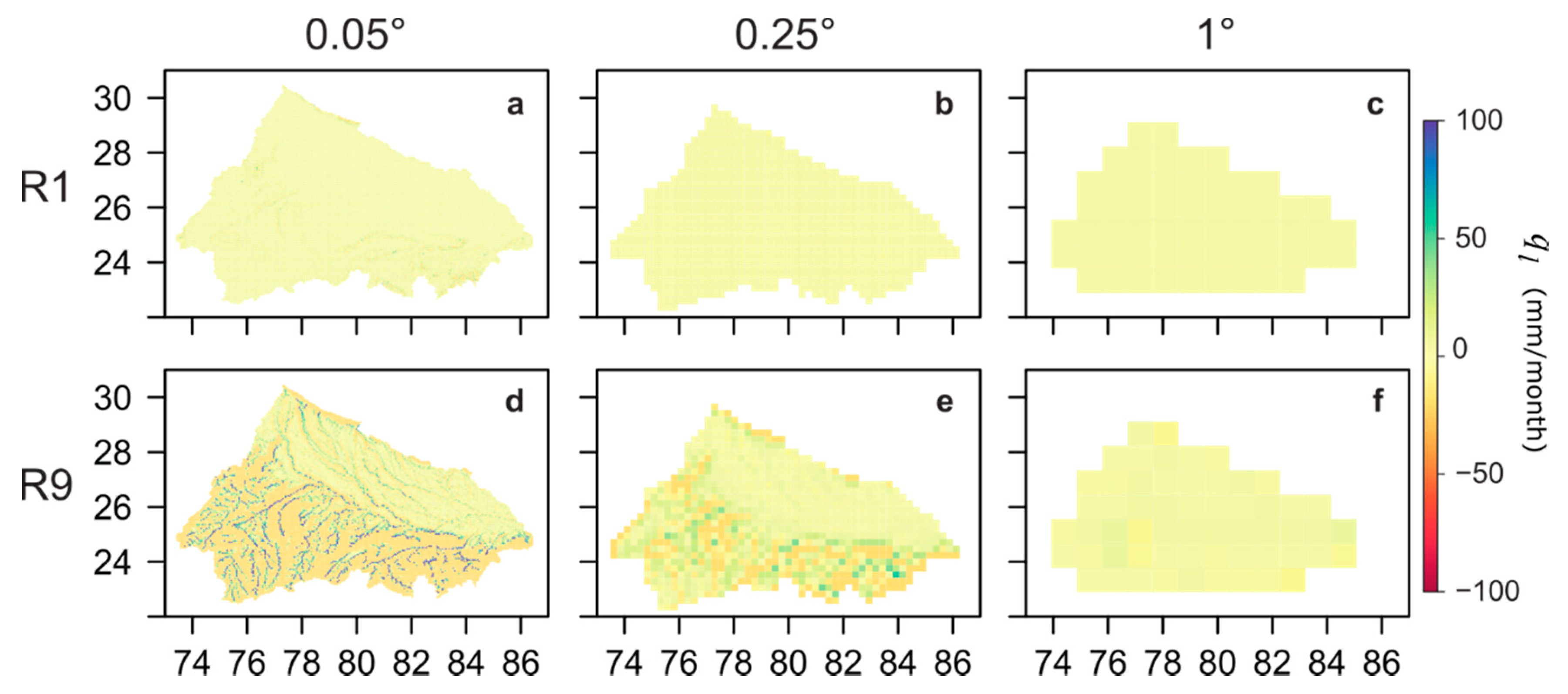
3.2.5. Lateral Groundwater Flow

We consider lateral groundwater flow, $q_l$, for each grid cell as defined by Krakauer et al. [58]: $q_l$

$$q_l=-q_r+S\frac{dh}{dt}$$

(7)

which is the net lateral groundwater flow, with negative values representing a net loss of groundwater from the cell. Cell-mean lateral groundwater flow consistently increases with decreasing model cell size and aquifer hydraulic conductivity (Table 3). Considering the median of the values of cell-mean lateral groundwater flow for all of the cells in the grid, q_l⁵⁰, then as the cell size decreases from 1 to 0.05, q_l⁵⁰ increases by 0.5, 4 and 13 mm/month for the low (R1), medium (R4) and high (R7) T aquifers, respectively. Similarly, the 99th percentile of this metric, q_l⁹⁹, increases by 12, 44 and 138 mm/month for the three aquifers.

Spatial variations in lateral groundwater flow are presented for the two runs R1 and R9, and the three different grid resolutions, in Figure 8. Cell-mean lateral groundwater flow for R1 and R9 and three different grid resolutions. For R1, the cell-mean lateral groundwater flow is very low, only increasing with increasing grid resolution from 0.02 to 1.43 mm/month on average. Lateral groundwater flow on the 0.05° grid for the low T aquifer (R1) is very localised, with cells with positive lateral flow being close to those with negative lateral flow; the water table interacts with the land surface across the majority of area, and therefore, whilst the hydraulic gradient is steep, the lateral flow is low. In contrast, for the high T aquifer run (R9), cell-mean lateral groundwater flow increases significantly with decreasing cell size: from 1.8 to 19.4 mm/month. In this run, lateral groundwater flow is positive in the river valleys, and negative over the upland interfluves.

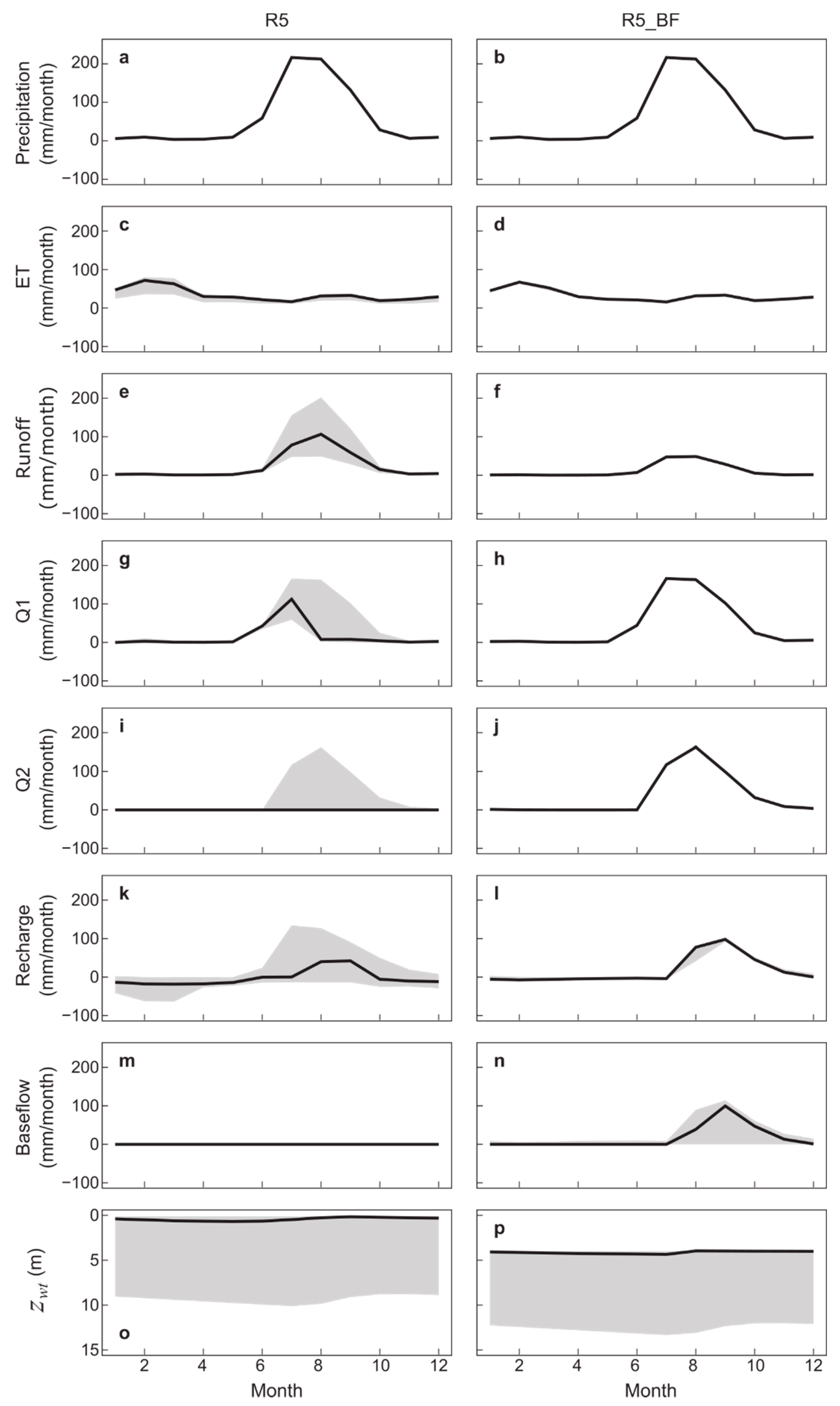
3.3. Comparison of Groundwater Discharge through Capillary Rise and River Baseflow

The discharge of groundwater to the land surface can occur via capillary rise through the soil, or through the river leakage mechanism where these boundaries are defined. To assess the maximum difference of both discharge mechanisms, we compare the two extreme cases, applying each discharge mechanism over the entire model domain. The variation over the annual cycle of cell-mean fluxes and WTD is compared in Figure 9 for the R5 and R5_BF runs on the 0.05°grid: in R5, groundwater discharges to the surface through the soil, and in R5_BF, groundwater discharges through the rivers boundaries via a groundwater head-dependent baseflow, when the water table rises to within zbase = 4 m of the land surface. In R5_BF, two components contribute to total runoff: that produced at the soil surface (Figure 9f), and that from baseflow to rivers (Figure 9n). In R5, runoff is only generated at the soil surface (Figure 9e).

Considering R5_BF first, the spatial variation in cell-mean ET, surface runoff and soil moisture fluxes is negligibly small because the WTD is limited to being greater than or equal to 4 m, as the stage of the river was set to 4 m below the surface in all cells, and the envelope of the 10th and 99th percentiles is very narrow. The delay in the peak of the flux as it propagates downwards through the soil layer and to baseflow discharge is also clear; the peak of the median of the cell baseflow time series in September occurs two months after that for surface runoff.

In contrast, the water table is shallower in R5 than R5_BF and within the soil column in low lying areas. The interaction of the groundwater table with the soil results in a spatial variation in soil moisture, surface runoff, ET, fluxes within the soil, and groundwater recharge. Groundwater recharge is predominantly downwards between July and September. In contrast, between October and July, water exchange with the groundwater table is predominantly in an upward direction due to capillary forces, which results in a higher median ET than for R5_BF: especially for January–March 54.8 mm/month (R5_BF) versus 60.3 mm/month (R5).

On average, recharge is larger for R5_BF (19.3 mm/month) than for R5 (13 mm/month), as in R5_BF the soil always drains to the 4 m or more deep water table. Total runoff, i.e., surface runoff plus baseflow, is slightly larger for the R5 (30.2 mm/month) than for the R5_BF (28.3 mm/month) model. This difference is because the water table for R5 is near the surface in the lowlands, resulting in reduced transpiration, and more runoff.

4. Discussion

The model simulations have been used to explore the magnitude of the changes in modelled state variables and fluxes as aquifer diffusivity and grid resolution are varied. The results show that changes in T produce more marked changes in modelled fluxes than changes in aquifer storage coefficient. This is because T controls the mean WTD, which in turn controls the vertical hydraulic gradient in the unsaturated zone and the soil moisture, which determine the recharge, ET and runoff rates. To further interpret the results, it is convenient to summarise the modelled fluxes as proportions of rainfall.

Table 4. Modelled mean fluxes as a percentage of mean rainfall between the low (R1), medium (R4) and high (R7) T models on the 0.05° grid.

	Low T (R1)	Medium T (R4)	High T (R7)	Change R1 to R7
WTD (m)	0.52	5.65	20.41	+19.89
Recharge (% rain)	20.6	21.3	27.8	+7.2
ET (% rain)	47.4	50.5	54.5	+7.1
Runoff (% rain)	51.8	48.7	44.7	−7.1
Lateral groundwater flow (% rain)	2.4	14.7	34.1	31.7
Discharge area fraction	0.63	0.51	0.29	−0.34

summarises the differences in the modelled WTD, mean fluxes as a percentage of mean rainfall, and discharge area fraction, between the low (R1), medium (R4) and high (R7) T models on the 0.05° grid.

Table 5. Changes in modelled variables as grid resolution is increased for 1° to 0.05°. Changes in fluxes are expressed as a percentage of the mean rainfall.

	Low T (R1)	Medium T (R4)	High T (R7)
WTD (m)	+0.2	+5.41	+20.11
Recharge (% rain)	−1.9	+7.0	+13.1
ET (% rain)	−1.4	+9.8	+12.3
Runoff (% rain)	+1.4	−9.8	−12.3
Lateral groundwater flow (% rain)	+2.4	+14.4	+31.2
Discharge area fraction	−0.04	−0.16	−0.33

summarises the changes in the same modelled variables for the same three models, as the grid resolution increases from 1° to 0.05°.

On the 0.05° grid, rainfall is partitioned approximately equally into ET and runoff. However, 7.1% more of the rainfall becomes ET in the high T model than the low T model. This is balanced by a 7.1% reduction in runoff. This is due to the more waterlogged soils and lower transpiration in the lower T simulations. In the low T model, 20.6% of the rainfall becomes recharge, which contributes to runoff via slow flow through the aquifer; subtracting this from the runoff indicates that 31.2% of the rainfall becomes rapid surface runoff generated by soil moisture excess. Recharge is 7.2% higher in the high T model than the low T model, due to the increase in mean WTD from 0.52 m to 20.41 m. Consequently, the surface (runoff minus recharge in Table 4) and subsurface (recharge in Table 4) components of runoff decrease and increase, respectively, to 16.9 and 27.8% of rainfall. As the mean WTD increases as T increases, the area generating upward groundwater discharge decreases from 63 to 29% of the catchment. Groundwater flow in the low T system is localised with only 2.4% of the rainfall moving laterally from a grid cell in which it formed recharge to a neighbouring model grid cell. This increases to 34.1% flowing laterally in the high T aquifer.

Considering all aquifer parameterisations, changes in the components of the model global flow balance as the grid resolution is increased from 1° to 0.05° vary between −1.4 and 13.1% of mean rainfall (Table 5). For the medium T model, the changes in the fluxes are similar to those produced by the hundred-fold increase in T in the 0.05° grid model. In the low T system, increasing the grid resolution has minimal effect as lateral groundwater flow is low, and the VIC grid cells behave as vertical columns. However, in the high T aquifer, increasing the grid resolution has a large impact of the cell water balances. More accurate simulation of the spatial distribution of water table elevations causes: runoff to decrease and ET to increase by 12.3% of the rainfall; lateral groundwater flow to increase to approximately one third of the rainfall; the area where recharge occurs to increase from around one third to two thirds of the catchment.

Snowdon et al. [59] have also recently shown the dependence of groundwater recharge and discharge on grid resolution when modelling shallow groundwater. Discretising a 715 km² catchment using grids ranging in resolution from 3 to 250 m, they similarly demonstrated that exchange flux magnitudes are sensitive to the hydraulic conductivity of the shallow bedrock and the hydraulic gradient, and therefore, that modelling at increasingly lower resolutions becomes subject to greater uncertainty. The importance of representing the contribution of groundwater to ET has also recently been shown to be important in [60,61], where it was demonstrated that shallow groundwater can buffer plant water stress as the climate warms. Similarly, the importance of groundwater on ET fluxes was found to be significant on the Iberian Peninsula, where ET was modelled to be 17.4% higher when a groundwater scheme was included compared to a simulation without groundwater [62].

Both grid size and transmissivity are important, as lateral groundwater flow distributes groundwater spatially within the catchment and moves water from areas with higher hydraulic head to discharge at lower lying areas. The maximum possible difference in hydraulic head is constrained by the maximum and minimum elevation within a sub-catchment, and therefore the averaging of the topography at increasing lower resolutions limits the hydraulic gradient. Krakauer et al. [58] compared grid spacing at a global scale and found that for a grid resolution of 0.1°, the magnitude of lateral groundwater flow was comparable to recharge. Krakauer et al. [58] further suggests that a model transitions from a state in which lateral flow contributes significantly to the cell water budget to it being insignificant as the modelled grid size increases from 0.1 and 1°. Therefore, Krakauer et al. [58] justify to some extent the neglection of lateral groundwater flow in current climate models.

However, as we have shown the impact of grid resolution on lateral groundwater flow also depends on the aquifer hydraulic properties, having little effect for low $T$ and a large effect for high $T$. Therefore, the efforts of modelling at a fine grid resolution becomes increasingly important when including lateral groundwater flow in catchments with a higher permeability. When considering the effects of groundwater abstraction, groundwater flow directions and magnitude can change within an aquifer and a high spatial grid resolution is likely to be important for all aquifer typologies.

The development of VIC to simulate lateral groundwater flow, and the effect of a dynamic water table on the exchange of water between the unsaturated zone and the saturated aquifer represents an important improvement in its representation of catchment hydrological processes. When addressing questions that are dependent on the WTD, such as representing groundwater abstraction and groundwater-fed irrigation, the depth to the water table needs to be represented adequately. However, we have implemented a relatively simple 2D groundwater model that simulates the aquifer using a single layer, which has to be connected to the soil column. Consequently, currently confined, leaky, and multi-layer aquifer systems cannot be modelled.

A VIC grid cell can be subdivided into a number of tiles, corresponding to different land cover types and elevation bands [21]; however, VIC has been tested here for one elevation band and vegetation type per grid cell. It is possible to include several vegetation types and elevation bands within a VIC cell, but there is only one water table elevation value per grid cell. An approach to include topographic subgrid variability, including that of the water table, has been developed by Choi et al. [63] within a three-dimensional soil moisture transport model. The study showed this to be an important factor controlling soil moisture dynamics and estimates of grid-scale surface energy fluxes. Subgrid variability for different plant functional types has been incorporated into a version of CLM 4.5 including lateral flow by using a finer groundwater model grid than the CLM model grid and distributing each plant functional type proportionally on the groundwater grid [27]. For future work, similar approaches could be added to this enhanced version of VIC. However, for the current version, we suggest the use of a consistently fine model grid for both VIC and the groundwater model, representing the variation in topography and vegetation for each grid cell.

In addition to improvement in model performance gained by increasing grid resolution, and thus a better representation of discharge areas alone, benefits can also accrue from the more detailed associated parameterisation. For example, Singh et al. [64] showed that for the land surface model CLM4.0, increasing the grid resolution from 100 to 1 km reduced errors between modelled and observed soil moisture, terrestrial water storage, sensible heat, and snow water equivalent. Using two groundwater models of New Zealand with different grid resolutions, Reinecke et al. [65] also showed improvements in modelled WTDs at higher spatial resolutions; however, this was also related to how groundwater level observations were aggregated within grid cells. They concluded that the density and range of observed values can vary greatly, which affects comparisons of models with different spatial resolutions. Furthermore, Reinecke et al. [65] showed that increasing the spatial resolution alone is not sufficient to simulate the hydraulic heads and the flows accurately, but that improvements in the modelled variation in the WTD can be achieved with a better representation of the spatial variation of aquifer properties, as previously considered by Westerhoff et al. [66]. Westerhoff et al. [66] refined the global scale equilibrium WTD model of Fan et al. [67] using higher resolution aquifer parameterisation, recharge, a fine model grid, and model calibration to observed groundwater levels, and this model simulated the WTD best compared to other global groundwater models in New Zealand [28,65,67]. Therefore, there is a need to update global hydrogeological parameterisations with local to national scale knowledge of aquifer properties, and include model calibration for a better representation of groundwater flows within large scale hydrological modelling.

Linking hydrological modelling with groundwater modelling is important, because it connects interconnected disciplines. As Staudinger et al. [68] discuss, often either hydrology or hydrogeology is resolved in more detail whilst simplifying the other system considerably. For example, hydrology examines the water cycle of the land surface, often applied to estimate floods or droughts, and treats the deeper subsurface as a boundary condition. In contrast hydrogeology simplifies the land surface processes and often prescribes a simplified groundwater recharge. By linking both hydrological and hydrogeological modelling, interactions and feedbacks between land surface processes and groundwater processes can be studied [68]. Therefore, the inclusion of lateral groundwater flow into a hydrological model allows the water cycle to be closed within a catchment, and lateral groundwater flow to transport water across grid cells of a hydrological model.

5. Conclusions

We have incorporated a two-dimensional groundwater flow model into the image version of VIC 5.0.1 [20]. We replaced the baseflow formulation in VIC, which is a function of soil moisture, with a vertical flux across the soil-aquifer boundary. This flux is based on the SIMGM model by Niu et al. [12], and includes both gravitational drainage and capillary rise. Depending on its sign, this flux across the soil-aquifer boundary can represent either groundwater recharge or groundwater discharge, and it is a function of the soil moisture and the current WTD simulated by the groundwater model. This enhanced version of the VIC model was applied to an idealised system of the upper Ganges, India, using a homogeneous parameterisation, except for the topographic elevation.

The magnitude of cell ET, runoff, groundwater recharge, and groundwater discharge rates significantly depend on WTD in the new VIC model, which in turn can be significantly affected by grid resolution. For the low (≤50 m²/day) transmissivity aquifer modelled, increasing the grid resolution from 1° to 0.05° has a minimal effect as lateral groundwater flow is low, and the VIC grid cells behave as vertical columns. However, in the medium (≤500 m²/day) and high (≤5000 m²/day) transmissivity systems, increasing the grid resolution resolves the water table distribution much more realistically, which has a large impact of the cell water balances. Decreasing the grid cell size from 1° to 0.05° causes mean ET and runoff to change by up to 12.3% of mean rainfall. For the medium transmissivity aquifer, changes in mean fluxes associated with the 20-fold increase in resolution are similar to those produced by hundred-fold variation in transmissivity in the highest resolution model. The frequency distribution of cell-mean water table depths is similar for the 0.25° high transmissivity model and the 0.05° medium transmissivity model. The relationship between WTD, model fluxes and grid resolution will, of course, differ for different aquifer types, climatic conditions, and topographic settings. However, because of the large variation of the WTD and cell fluxes with grid cell size in this application, we suggest that such an analysis should be undertaken as part of the model’s calibration process.

The inclusion of a groundwater model in VIC facilitates the inclusion of human processes, such as groundwater abstraction and irrigation, which will be the focus of future development. This will improve the representation of feedbacks between water use and terrestrial water storage leading to, for example, better understanding of how ET and river flows are affected by the practice of groundwater-fed irrigation.

References

1. Nazemi, A.; Wheater, H.S. On inclusion of water resource management in Earth system models -Part 1: Problem definition and representation of water demand. Hydrol. Earth Syst. Sci. 2015, 19, 33–61. [Google Scholar] [CrossRef] [Green Version]
2. Wada, Y.; Bierkens, M.F.P.; De Roo, A.; Dirmeyer, P.A.; Famiglietti, J.S.; Hanasaki, N.; Konar, M.; Liu, J.; Schmied, H.M.; Oki, T.; et al. Human-water interface in hydrological modelling: Current status and future directions. Hydrol. Earth Syst. Sci. 2017, 21, 4169–4193. [Google Scholar] [CrossRef] [Green Version]
3. Taylor, R.G.; Scanlon, B.; Döll, P.; Rodell, M.; van Beek, R.; Wada, Y.; Longuevergne, L.; Leblanc, M.; Famiglietti, J.S.; Edmunds, M.; et al. Ground water and climate change. Nat. Clim. Chang. 2012, 3, 322. [Google Scholar] [CrossRef] [Green Version]
4. Condon, L.E.; Maxwell, R.M. Groundwater-fed irrigation impacts spatially distributed temporal scaling behavior of the natural system: A spatio-temporal framework for understanding water management impacts. Environ. Res. Lett. 2014, 9, 034009. [Google Scholar] [CrossRef]
5. Leng, G.; Huang, M.; Tang, Q.; Gao, H.; Leung, L.R. Modeling the effects of groundwater-fed irrigation on terrestrial hydrology over the conterminous United States. J. Hydrometeorol. 2014, 15, 957–972. [Google Scholar] [CrossRef]
6. Nazemi, A.; Wheater, H.S. On inclusion of water resource management in Earth system models Part 2: Representation of water supply and allocation and opportunities for improved modeling. Hydrol. Earth Syst. Sci. 2015, 19, 63–90. [Google Scholar] [CrossRef] [Green Version]
7. Siebert, S.; Döll, P.; Hoogeveen, J.; Faures, J.M.; Frenken, K.; Feick, S. Development and validation of the global map of irrigation areas. Hydrol. Earth Syst. Sci. 2005, 9, 535–547. [Google Scholar] [CrossRef]
8. Pokhrel, Y.N.; Koirala, S.; Yeh, P.J.F.; Hanasaki, N.; Longuevergne, L.; Kanae, S.; Oki, T. Incorporation of groundwater pumping in a global Land Surface Model with the representation of human impacts. Water Resour. Res. 2015, 51, 78–96. [Google Scholar] [CrossRef] [Green Version]
9. Keune, J.; Sulis, M.; Kollet, S.; Siebert, S.; Wada, Y. Human Water Use Impacts on the Strength of the Continental Sink for Atmospheric Water. Geophys. Res. Lett. 2018, 45, 4068–4076. [Google Scholar] [CrossRef]
10. MacDonald, A.M.; Bonsor, H.C.; Ahmed, K.M.; Burgess, W.G.; Basharat, M.; Calow, R.C.; Dixit, A.; Foster, S.S.D.; Gopal, K.; Lapworth, D.J.; et al. Groundwater quality and depletion in the Indo-Gangetic Basin mapped from in situ observations. Nat. Geosci. 2016, 9, 762–766. [Google Scholar] [CrossRef]
11. Döll, P.; Mueller Schmied, H.; Schuh, C.; Portmann, F.T.; Eicker, A. Global-scale assessment of groundwater depletion and related groundwater abstractions: Combining hydrological modeling with information from well observations and GRACE satellites. Water Resour. Res. 2014, 50, 5698–5720. [Google Scholar] [CrossRef]
12. Niu, G.Y.; Yang, Z.L.; Dickinson, R.E.; Gulden, L.E.; Su, H. Development of a simple groundwater model for use in climate models and evaluation with Gravity Recovery and Climate Experiment data. J. Geophys. Res. Atmos. 2007, 112, D07103. [Google Scholar] [CrossRef]
13. Rosenberg, E.A.; Clark, E.A.; Steinemann, A.C.; Lettenmaier, D.P. On the contribution of groundwater storage to interannual streamflow anomalies in the Colorado River basin. Hydrol. Earth Syst. Sci. 2013, 17, 1475–1491. [Google Scholar] [CrossRef] [Green Version]
14. Yeh, P.J.F.; Eltahir, E.A.B. Representation of Water Table Dynamics in a Land Surface Scheme. Part I: Model Development. J. Clim. 2005, 18, 1861–1880. [Google Scholar] [CrossRef]
15. Maxwell, R.M.; Miller, N.L. Development of a coupled land surface and groundwater model. J. Hydrometeorol. 2005, 6, 233–247. [Google Scholar] [CrossRef] [Green Version]
16. Yang, H.W.; Xie, Z.H. A new method to dynamically simulate groundwater table in land surface model VIC. Prog. Nat. Sci. 2003, 13, 819–825. [Google Scholar] [CrossRef]
17. Ruiz, L.; Varma, M.R.R.; Kumar, M.S.M.; Sekhar, M.; Maréchal, J.-C.; Descloitres, M.; Riotte, J.; Kumar, S.; Kumar, C.; Braun, J.-J. Water balance modelling in a tropical watershed under deciduous forest (Mule Hole, India): Regolith matric storage buffers the groundwater recharge process. J. Hydrol. 2010, 380, 460–472. [Google Scholar] [CrossRef] [Green Version]
18. Chang, L.-L.; Dwivedi, R.; Knowles, J.F.; Fang, Y.-H.; Niu, G.-Y.; Pelletier, J.D.; Rasmussen, C.; Durcik, M.; Barron-Gafford, G.A.; Meixner, T. Why Do Large-Scale Land Surface Models Produce a Low Ratio of Transpiration to Evapotranspiration? J. Geophys. Res. Atmos. 2018, 123, 9109–9130. [Google Scholar] [CrossRef]
19. Chawla, I.; Mujumdar, P.P. Isolating the impacts of land use and climate change on streamflow. Hydrol. Earth Syst. Sci. 2015, 19, 3633–3651. [Google Scholar] [CrossRef] [Green Version]
20. Hamman, J.J.; Nijssen, B.; Bohn, T.J.; Gergel, D.R.; Mao, Y.X. The Variable Infiltration Capacity model version 5 (VIC-5): Infrastructure improvements for new applications and reproducibility. Geosci. Model. Dev. 2018, 11, 3481–3496. [Google Scholar] [CrossRef] [Green Version]
21. Liang, X.; Lettenmaier, D.P.; Wood, E.F.; Burges, S.J. A simple hydrologically based model of land surface water and energy fluxes for general circulation models. J. Geophys. Res. 1994, 99, 14,415–414,428. [Google Scholar] [CrossRef]
22. Mishra, V.; Shah, R.; Azhar, S.; Shah, H.; Modi, P.; Kumar, R. Reconstruction of droughts in India using multiple land-surface models (1951–2015). Hydrol. Earth Syst. Sci. 2018, 22, 2269–2284. [Google Scholar] [CrossRef] [Green Version]
23. Shah, R.; Sahai, A.K.; Mishra, V. Short to sub-seasonal hydrologic forecast to manage water and agricultural resources in India. Hydrol. Earth Syst. Sci. 2017, 21, 707–720. [Google Scholar] [CrossRef] [Green Version]
24. Madhusoodhanan, C.G.; Sreeja, K.G.; Eldho, T.I. Assessment of uncertainties in global land cover products for hydro-climate modeling in India. Water Resour. Res. 2017, 53, 1713–1734. [Google Scholar] [CrossRef]
25. Fan, Y.; Miguez-Macho, G.; Weaver, C.P.; Walko, R.; Robock, A. Incorporating water table dynamics in climate modeling: 1. Water table observations and equilibrium water table simulations. J. Geophys. Res. Atmos. 2007, 112, D10125. [Google Scholar] [CrossRef]
26. Miguez-Macho, G.; Fan, Y.; Weaver, C.P.; Walko, R.; Robock, A. Incorporating water table dynamics in climate modeling: 2. Formulation, validation, and soil moisture simulation. J. Geophys. Res. Atmos. 2007, 112, D13108. [Google Scholar] [CrossRef] [Green Version]
27. Zeng, Y.; Xie, Z.; Liu, S.; Xie, J.; Jia, B.; Qin, P.; Gao, J. Global Land Surface Modeling Including Lateral Groundwater Flow. J. Adv. Modeling Earth Syst. 2018, 10, 1882–1900. [Google Scholar] [CrossRef]
28. de Graaf, I.E.M.; Sutanudjaja, E.H.; Van Beek, L.P.H.; Bierkens, M.F.P. A high-resolution global-scale groundwater model. Hydrol. Earth Syst. Sci. 2015, 19, 823–837. [Google Scholar] [CrossRef] [Green Version]
29. de Graaf, I.E.M.; van Beek, R.L.P.H.; Gleeson, T.; Moosdorf, N.; Schmitz, O.; Sutanudjaja, E.H.; Bierkens, M.F.P. A global-scale two-layer transient groundwater model: Development and application to groundwater depletion. Adv. Water Resour. 2017, 102, 53–67. [Google Scholar] [CrossRef]
30. Sutanudjaja, E.H.; Van Beek, R.; Wanders, N.; Wada, Y.; Bosmans, J.H.C.; Drost, N.; Van Der Ent, R.J.; De Graaf, I.E.M.; Hoch, J.M.; De Jong, K.; et al. PCR-GLOBWB 2: A 5 arcmin global hydrological and water resources model. Geosci. Model. Dev. 2018, 11, 2429–2453. [Google Scholar] [CrossRef] [Green Version]
31. Harbaugh, A. MODFLOW-2005, The U.S. Geological Survey Modular Ground-Water Model.—The Ground-Water Flow Process.; U.S. Geological Survey Techniques and Methods 6-A16; U.S. Geological Survey: Reston, VA, USA, 2005. [CrossRef] [Green Version]
32. Sridhar, V.; Billah, M.M.; Hildreth, J.W. Coupled Surface and Groundwater Hydrological Modeling in a Changing Climate. Groundwater 2018, 56, 618–635. [Google Scholar] [CrossRef]
33. Kang, H.; Sridhar, V. Drought assessment with a surface-groundwater coupled model in the Chesapeake Bay watershed. Environ. Model. Softw. 2019, 119, 379–389. [Google Scholar] [CrossRef]
34. Brandmeyer, J.E.; Karimi, H.A. Coupling methodologies for environmental models. Environ. Model. Softw. 2000, 15, 479–488. [Google Scholar] [CrossRef]
35. Franchini, M.; Pacciani, M. Comparative analysis of several conceptual rainfall-runoff models. J. Hydrol. 1991, 122, 161–219. [Google Scholar] [CrossRef]
36. Foster, T.; Brozović, N.; Butler, A.P. Modeling irrigation behavior in groundwater systems. Water Resour. Res. 2014, 50, 6370–6389. [Google Scholar] [CrossRef] [Green Version]
37. Frija, A.; Chebil, A.; Speelman, S. Farmers’ Adaptation to Groundwater Shortage in the Dry Areas: Improving Appropriation or Enhancing Accommodation? Irrig. Drain. 2016, 65, 691–700. [Google Scholar] [CrossRef]
38. O’Keeffe, J.; Buytaert, W.; Mijic, A.; Brozović, N.; Sinha, R. The use of semi-structured interviews for the characterisation of farmer irrigation practices. Hydrol. Earth Syst. Sci. 2016, 20, 1911–1924. [Google Scholar] [CrossRef] [Green Version]
39. O’Keeffe, J.; Moulds, S.; Bergin, E.; Brozović, N.; Mijic, A.; Buytaert, W. Including Farmer Irrigation Behavior in a Sociohydrological Modeling Framework With Application in North India. Water Resour. Res. 2018, 54, 4849–4866. [Google Scholar] [CrossRef]
40. Shah, T.; Singh, O.P.; Mukherji, A. Some aspects of South Asia’s groundwater irrigation economy: Analyses from a survey in India, Pakistan, Nepal Terai and Bangladesh. Hydrogeol. J. 2006, 14, 286–309. [Google Scholar] [CrossRef]
41. Wood, E.F.; Lettenmaier, D.P.; Zartarian, V.G. A land-surface hydrology parameterization with subgrid variability for general circulation models. J. Geophys. Res. 1992, 97, 2717–2728. [Google Scholar] [CrossRef]
42. Gao, H.; Tang, Q.; Shi, X.; Zhu, C.; Bohn, T.J.; Su, F.; Sheffield, J.; Pan, M.; Lettenmaier, D.P.; Wood, E.F. Water Budget Record from Variable Infiltration Capacity (VIC) Model. Algorithm Theor. Basis Doc. Terr. Water Cycle Data Rec. 2010. (in review). [Google Scholar]
43. Lohmann, D.; Nolte-Holube, R.; Raschke, E. A large-scale horizontal routing model to be coupled to land surface parametrization schemes. Tellusseries A: Dyn. Meteorol. Oceanogr. 1996, 48, 708–721. [Google Scholar] [CrossRef]
44. Tomer, S.; Muddu, S.S.; Mehta, V.K.; Yegina, S.; Thiyaku, S. Package ‘ambhasGW’. Available online: https://cran.r-project.org/web/packages/ambhasGW/index.html (accessed on 2 December 2020).
45. Wang, H.F.; Anderson, M.P. Introduction to Groundwater Modeling: Finite Difference and Finite Element Methods; Academic Press: San Diego, CA, USA, 1995. [Google Scholar]
46. Holden, H.; Karlsen, K.H.; Lie, K.-A. Splitting Methods for Partial Differential Equations with Rough Solutions: Analysis and MATLAB Programs; European Mathematical Society Series of Lectures in Mathematics. 2010, Volume 11. Available online: https://bookstore.ams.org/emsserlec-11 (accessed on 2 December 2020).
47. Smith, G.D.; Smith, G.D.; Smith, G.D.S. Numerical Solution of Partial Differential Equations: Finite Difference Methods; Oxford University Press: Oxford, UK, 1985. [Google Scholar]
48. Kiehl, J.T.; Gent, P.R. The community climate system model, version 2. J. Clim. 2004, 17, 3666–3682. [Google Scholar] [CrossRef] [Green Version]
49. Campbell, G.S. Soil Physics with BASIC: Transport. Models for Soil-Plant. Systems; Elsevier: Amsterdam, The Netherlands, 1985; Volume 14. [Google Scholar]
50. DHI, M. FEFLOW 7.0 User Guide; DHI: Copenhagen, Denmark, 2016. [Google Scholar]
51. Jackson, C.; Spink, A. User’s Manual for the Groundwater Flow Model ZOOMQ3D; IR/04/140; British Geological Survey: Keyworth, UK, 2004.
52. Miguez-Macho, G.; Fan, Y. The role of groundwater in the Amazon water cycle: 1. Influence on seasonal streamflow, flooding and wetlands. J. Geophys. Res. Atmos. 2012, 117, D15113. [Google Scholar] [CrossRef]
53. Hiscock, K. Hydrogeology: Principles and Practice; Blackwell Science Ltd.: Oxford, UK, 2005. [Google Scholar]
54. Jarvis, A.; Reuter, H.I.; Nelson, A.; Guevara, E. Hole-Filled SRTM for the Globe Version 4; CGIAR-CSI SRTM 90 m Database. Available online: http://srtm.csi.cgiar.org/ (accessed on 2 December 2020).
55. Mazumder, R.; Eriksson, P.G. Chapter 1 Precambrian basins of India: Stratigraphic and tectonic context. Geol. Soc. Lond. Mem. 2015, 43, 1. [Google Scholar] [CrossRef] [Green Version]
56. Nijssen, B.; Schnur, R.; Lettenmaier, D.P. Global Retrospective Estimation of Soil Moisture Using the Variable Infiltration Capacity Land Surface Model, 1980–1993. J. Clim. 2001, 14, 1790–1808. [Google Scholar] [CrossRef]
57. Weedon, G.P.; Gomes, S.; Viterbo, P.; Österle, H.; Adam, J.C.; Bellouin, N.; Boucher, O.; Best, M. The WATCH forcing data 1958-2001: A Meteorological Forcing Dataset for Land Surface- and Hyrological-Models. Available online: https://catalogue.ceh.ac.uk/documents/ba6e8ddd-22a9-457d-acf4-d63cd34f2dda (accessed on 2 December 2020).
58. Krakauer, N.Y.; Li, H.; Fan, Y. Groundwater flow across spatial scales: Importance for climate modeling. Environ. Res. Lett. 2014, 9, 034003. [Google Scholar] [CrossRef]
59. Snowdon, A.P.; Sykes, J.F.; Normani, S.D. Topography scale effects on groundwater-surface water exchange fluxes in a Canadian Shield setting. J. Hydrol. 2020, 585, 124772. [Google Scholar] [CrossRef]
60. Condon, L.E.; Atchley, A.L.; Maxwell, R.M. Evapotranspiration depletes groundwater under warming over the contiguous United States. Nat. Commun. 2020, 11, 873. [Google Scholar] [CrossRef]
61. Marchionni, V.; Daly, E.; Manoli, G.; Tapper, N.J.; Walker, J.P.; Fatichi, S. Groundwater Buffers Drought Effects and Climate Variability in Urban Reserves. Water Resour. Res. 2020, 56, e2019WR026192. [Google Scholar] [CrossRef]
62. Martínez-de la Torre, A.; Miguez-Macho, G. Groundwater influence on soil moisture memory and land–atmosphere fluxes in the Iberian Peninsula. Hydrol. Earth Syst. Sci. 2019, 23, 4909–4932. [Google Scholar] [CrossRef] [Green Version]
63. Choi, H.I.; Kumar, P.; Liang, X.-Z. Three-dimensional volume-averaged soil moisture transport model with a scalable parameterization of subgrid topographic variability. Water Resour. Res. 2007, 43, W04414. [Google Scholar] [CrossRef] [Green Version]
64. Singh, R.S.; Reager, J.T.; Miller, N.L.; Famiglietti, J.S. Toward hyper-resolution land-surface modeling: The effects of fine-scale topography and soil texture on CLM4.0 simulations over the Southwestern U.S. Water Resour. Res. 2015, 51, 2648–2667. [Google Scholar] [CrossRef] [Green Version]
65. Reinecke, R.; Wachholz, A.; Mehl, S.; Foglia, L.; Niemann, C.; Döll, P. Importance of spatial resolution in global groundwater modeling. Groundwater 2020, 58, 363–376. [Google Scholar] [CrossRef] [Green Version]
66. Westerhoff, R.; White, P.; Miguez-Macho, G. Application of an improved global-scale groundwater model for water table estimation across New Zealand. Hydrol. Earth Syst. Sci. 2018, 22, 6449–6472. [Google Scholar] [CrossRef] [Green Version]
67. Fan, Y.; Li, H.; Miguez-Macho, G. Global patterns of groundwater table depth. Science 2013, 339, 940–943. [Google Scholar] [CrossRef] [Green Version]
68. Staudinger, M.; Stoelzle, M.; Cochand, F.; Seibert, J.; Weiler, M.; Hunkeler, D. Your work is my boundary condition!: Challenges and approaches for a closer collaboration between hydrologists and hydrogeologists. J. Hydrol. 2019, 571, 235–243. [Google Scholar] [CrossRef]
Figure 1. Layering in coupled soil-aquifer column and vertical variation in storage coefficient S . Z 1 , Z 2 , Z 3 are the node depths of the variable infiltration capacity (VIC) soil column, Z b o t is the elevation of the bottom layer in VIC, Z w t the water table depth, and Z b a s e the elevation of the base of the aquifer.
Water 13 00663 g001
Figure 2. Model extent and SRTM land surface elevation data [54] aggregated to the three model grid resolutions.
Water 13 00663 g002
Figure 3. Daily average temperature and precipitation for the period 1979 to 2002, using WATCH climatology [57].
Water 13 00663 g003
Figure 4. Mean values of water table depth (af), groundwater recharge (gl), ET (mr), and runoff (sx) for R1 (low T , low S ) and R9 (high T , high S ) models, and three grid resolutions 0.05°, 0.25° and 1°.
Water 13 00663 g004
Figure 5. Groundwater recharge and discharge, ET, and runoff against WTD (a,e,i,m), and density distributions of cell-mean fluxes for these four variables over annual (b,f,j,n), July–September (JAS) (c,g,k,o), and January–March (JFM) (d,h,l,p) periods for different aquifer parameterisations. The dotted line in (a,e,i,m) represents the depth of the soil layers. Note the broken axis on 10 of the plots.
Water 13 00663 g005
Figure 6. Cumulative distribution functions of cell-mean WTD at three different grid resolutions for the low, medium and high transmissivity models.
Water 13 00663 g006
Figure 7. Distributions of water table depth and cell-mean fluxes for different grid resolutions and aquifer parameterisations. Note the broken axis (c,e).
Water 13 00663 g007
Figure 8. Cell-mean lateral groundwater flow for R1 and R9 and three different grid resolutions.
Water 13 00663 g008
Figure 9. Time series of cell fluxes for: the R5 model in which all groundwater discharge occurs through interaction with the land surface, and the R5_BF model including groundwater head-dependent baseflow. Precipitation is that reaching the soil surface, Q1 is the flux between soil layers 1 and 2, Q2 is the flux between soil layers 2 and 3, baseflow is the river baseflow contribution for R5_BF. The solid line is the median of the model cell values and the shaded area is the range within the 10–90% tile.
Water 13 00663 g009